A systematic framework for assessing discounts [Founders Pledge]
How do experimental effects translate to the real-world?
This report aims to provide guidelines for producing discounts within cost-effectiveness analyses; how to take an effect size from an RCT and apply discounts to best predict the real-world effect of an intervention. The goal is to have guidelines that produce accurate estimates, and are practical for researchers to use. These guidelines are likely to be updated further, and I especially invite suggestions and criticism for the purpose of further improvement. A google docs version of this report is available here.
Acknowledgements: I would like to thank Matt Lerner, Filip Murár, David Reinstein and James Snowden for helpful comments on this report. I would also like to thank the rest of the FP research team for helpful comments during a presentation on this report.
Summary
This document provides guidelines for estimating the discounts that we (Founders Pledge) apply to RCTs in our cost-effectiveness analyses for global health and development charities. To skip directly to these guidelines, go to the ‘Guidance for researchers’ sections (here, here and here; separated by each type of discount).
I think that we should separate out discounts into internal reliability and external validity adjustments, because these components have different causes (see Fig 1.)
For internal reliability (degree to which the study accurately assesses the intervention in the specific context of the study- aka if an exact replication of the study was carried out, would we see the same effect?);
All RCTs will need a Type M adjustment; an adjustment that corrects for potential inflation of effect size (Type M error). The RCTs that are likely to have the most inflated effect sizes are those that are low powered (where the statistical test used has only a small chance of successfully detecting an effect, see more info here), especially if they are providing some of the first evidence for the effect. Factors to account for include publication bias, researcher bias (e.g. motivated reasoning to find an exciting result; running a variety of statistical tests and only reporting the ones that reach statistical significance would be an example of this), and methodological errors (e.g. inadequate randomisation of test trial subjects). See here for guidelines, and here to assess power.
Many RCTs are likely to need a 50-60% Type M discount, but there is a lot of variation here; table 1 can help to sense-check Type M adjustments.
A small number (<~15%) of RCTs will need a Type S adjustment, to account for the possibility that the sign of the effect is in the wrong direction. This is for RCTs that are producing some of the first evidence for an effect, are underpowered, and where it is mechanistically plausible that the effect could go in the other direction. See here for guidelines.
The likelihood of Type S error can be estimated mathematically (e.g. via the retrodesign R package).
For external validity (how that result generalises to a different context, e.g. when using an RCT effect size to estimate how well an intervention will work in a different area), we should expect that the absolute median effect size will vary between different contexts by around 99% (so a 1X effect size could be as little as ~0X or ~2X in a different context; see Vivalt 2020). Note that the effect in the new context could be larger than our estimate of the true effect, but I expect that in most cases it will be smaller. Following Duflo & Banerjee (2017), we should attend to;
Specific sample differences (do the conditions necessary for the intervention to work hold in the new context?)
Equilibrium effects (will there be emergent effects of the intervention, when carried out at scale?)
Special care effects (will the program be carried out differently when at scale, relative to the RCT?)
While this work focuses upon RCTs, these guidelines should be broadly applicable to quasi-experimental work. However, working out discounts for quasi-experimental work will additionally entail examining whether the experiment’s methodological assumptions are met (see here).
This report is laid out with a focus on the guidelines for researchers. However, for readers seeking a deeper understanding of the empirical evidence and reasoning that has gone into these guidelines, please go to ‘Notes on relevant papers’ within the Appendix.
These guidelines are a work in progress, and I expect them to be further developed/refined. Criticism and feedback are encouraged.
Fig 1: Diagram of the factors which influence the degree to which we should expect that an RCT result will generalise to a new context, separated by internal versus external validity.
Introduction
At Founders Pledge, we use cost-effectiveness analyses to predict the impact of particular interventions or charities per amount of money that is donated. This entails estimating the likely impact of a given intervention. For example, how strongly does an anti-malarial net affect mortality, or a deworming pill affect future income? Within our analyses of interventions related to global health and development, our estimates of these impacts usually come from randomised controlled trials (RCTs) or quasi-experimental studies. However, these effect sizes might not accurately represent the true effect that we would actually observe from a particular intervention. For example, effect sizes reported in an RCT may be inflated due to bias or a lack of statistical power. In addition, effect sizes that were found in one context might not be representative of the effects that we should expect in a new context. To account for these issues, we usually apply discounts to RCT/ quasi-experimental results within our cost-effectiveness analyses. The purpose of this work is to assess the degree to which these results replicate and generalize, in order to better standardise our processes for estimating these discounts.
Replicability and generalisability are easy to conflate. Replicability (in the context in which we use it) refers to whether an RCT would replicate, if it were to be rerun; to what extent does the study provide strong evidence for its findings? Generalisability refers to whether RCT results will generalise to new contexts; will the same intervention work, in a new area? It is possible that an RCT with excellent replicability will have poor generalisability. I have therefore split up these discounts into two components; internal reliability (corresponding to replicability) and external validity (referring to generalisability; see Fig 1). Since these two aspects of validity have different causes, I suggest that we should structure our discounts in this manner— this also matches GiveWell’s approach.
Following Gelman and Carlin (2014), I split internal reliability itself into two components. First is the Type M error, or whether the magnitude of the effect size is correct. Second is the Type S error, or the probability that the study’s measured effect is in the wrong direction. I chose this distinction because it does not rely upon p-values, as we move towards increasingly Bayesian methods (for criticism of p-values, see (Burnham & Anderson, 2014; Ellison, 2004; Gardner & Altman, 1986). At the same time, this approach is generally compatible with existing literature which uses null hypothesis testing and p-values. In the case of Type M errors, I argue that we can estimate effect size inflation by examining statistical power and likelihood of bias. I argue that Type S errors are likely to be fairly uncommon for the type of studies that we typically work with, but will need to be accounted for in certain situations. Overall, I estimate that the median effect size (that we might use in our CEAs) is likely to require an internal reliability Type M adjustment of ~50-60%. However, I highlight that there is also a lot of variation here.
A theme that underlies this internal reliability work—and that I suspect has been previously underappreciated—is the importance of statistical power, and its interaction with publication bias in generating inflated effect sizes. Power is the ability of a statistical test to correctly detect an effect, assuming that it is there. While low power is well known to increase the rates of false negatives, it is less well-appreciated that low power also increases effect size inflation (when conditioned upon statistical significance; Button et al., 2013; Gelman and Carlin 2014). This is because underpowered studies will tend to only successfully identify that an effect is present when the effect size is inflated, for example due to random error (see Question 2 for full explanation). My best understanding is that this effect underlies a large amount of replicability variation across experimental work. The upside to this is that we can get quite far (in determining the likely inflation of an effect size) by attending to study power. The downside is that it is often difficult to calculate a study’s power—it is possible that the approach outlined here will prove impractical—although I have created some guidelines and rules-of-thumb below.
A second theme that underlies this work is the importance of forming baseline estimates of the likely effect of an intervention, independent of the study at hand. We should be somewhat skeptical of ‘surprising’ results—interventions that appear to work well (according to the effect size), but their mechanism is poorly understood. Perhaps unsurprisingly, the rate of false positives in the experimental literature is higher when researchers investigate hypotheses with lower prior odds of being true (Ioannidis, 2005). In line with the idea that forming baseline estimates is important, note that while replication studies have frequently indicated that studies frequently fail to replicate (e.g. Camerer et al., 2016; Open Science Collaboration, 2015), people do appear to be reasonably good at predicting which studies will replicate. For example, Forsell et al. (2019) found that prediction markets correctly predicted 75% of replication outcomes among 24 psychology replications—although people were less willing to make predictions about effect sizes. As these efforts proceed, I think it will be possible in the future to use people’s predictions to form our baseline estimates of whether given interventions tend to work (e.g. on the Social Science Prediction Platform).
External validity refers to the extent to which an RCT/ quasi-experimental result will generalise, if the same study is undertaken in a different context. Although I view external validity as being probably more critical than internal reliability in determining an intervention’s success, there is a far smaller amount of relevant evidence here. I take the view that we should approach this question mechanistically, by examining (1) the extent to which the conditions required for the intervention to work hold in the new context (note that we should expect some RCTs will have effects going in the opposite direction when tested in a new context); (2) whether the effect in the RCT was larger due to participants realising that they were being watched (social desirability biases); (3) whether there are emergent effects from the intervention that will appear once it is scaled up, and; (4) whether the intervention will be conducted in a different way (i.e. less rigorously) when completed at scale (see; Duflo & Banerjee, 2017). Existing empirical work can ground our estimates. For example, Vivalt’s (2020) work suggests that the median absolute amount by which a predicted effect size differs from the same value given in a different study is approximately 99%. In addition, I have created a library of our current discounts here so that researchers can compare their discounts relative to others.
As a note, I have only briefly considered quasi-experimental evidence within this work, and have generally focused upon RCTs. Many of the points covered in this write-up will also apply to quasi-experimental work, but researchers assessing quasi-experimental studies will need to spend longer on assessing methodological bias relative to the guidelines suggested here for an RCT (e.g. establishing causation; see here).
Overall, this work aims to create clearer frameworks for estimating the appropriate discounts for RCTs. I think that this work is unlikely to affect well-studied interventions (which have high power anyway), and is likely to be most helpful for establishing discounts for ‘risky’ interventions that are comparatively less well-studied.
Internal reliability
internal reliability is the extent to which a given study supports the claims that it is making. If an exact replication of the study was carried out, would we see the same effect? Studies that are poorly designed, for instance with a low sample size, are likely to have lower internal reliability. If the effect size for a given study is inflated or in the wrong direction in the first place, it is unlikely that this intervention will have a beneficial effect when scaled to a new area.
I have split internal reliability into two components; Type S and Type M error (Gelman & Carlin, 2014). Both components can be estimated by attending to similar features of the data; whether the study is sufficiently well-powered, how large the standard errors are, the potential for bias within the study, and the prior expectation (independent of the particular study that is being examined) for the presence and magnitude of the effect. I go through these aspects in more detail below, before estimating the overall magnitude of Type M errors/ baseline rate of Type S error in the context of producing CEAs.
Estimating Type M and Type S errors requires estimating statistical power; the probability that the hypothesis test used will successfully identify an effect, if there is an effect to be found. Note that power in studies is often very low. Despite the convention of considering 80% power to be appropriate, reviews from across the medical, economic and general social science literature suggest that power is usually far lower than this (Button et al., 2013; Coville & Vivalt, 2017; Ioannidis et al., 2017). For example, in psychology a large survey of 200 meta-analyses (covering ~8000 articles) suggests that the median power is around 36%, with only ~8% of studies having adequate power (using Cohen’s 80% convention) (Stanley et al., 2018). Similarly, it has recently been estimated that the median power in political science articles is ~10%, with only ~10% of studies having adequate power. In economics, median power is ~18%, with around 10% of studies having adequate power (Ioannidis et al., 2017).
Q1: How large should we expect Type M errors to be?
We can predict that published papers will have (on average) larger effect sizes than the true effect size for a given intervention. This is due to a combination of low statistical power and bias. One way to get an estimate of the size of these effects is to look at the difference between effect sizes reported in pre-registered and well-powered replication studies versus original studies (see studies listed below). Unlike the original studies, these estimates should be relatively unaffected by publication bias.
Type M error is strongly affected by the power of the study, and the presence of publication bias. As a rule of thumb, the lower the power of the study, the more inflated the effect size is likely to be if the threshold of statistical significance (<0.05) was reached. This is due to an effect called the ‘winner’s curse’ (see Fig 9), and is liable to occur whenever there is a benchmark statistical significance level to be reached. For example, imagine that an effect really exists with an effect size of 0.2. Our study only has the power to detect this effect size 20% of the time. The results of any study are subject to sampling variation and random error, meaning that the study could hypothetically find an effect size that is either smaller or larger; say 0.1 or 0.3. However, due to low power, the study does not successfully detect the 0.1 or 0.2 effect sizes; only the third case (0.3) reaches statistical significance. The ‘winner’s curse’ means that the filter of 0.05 significance level means that the under-powered studies will only tend to find statistically significant results when the ‘lucky experimenters’ happened to obtain an effect size that is inflated due to random error (Button et al., 2013). Because statistically significant results are more likely to be published, this means that there is an overrepresentation in the literature of larger effect sizes at p values < 0.05. We should be most worried about winner’s curse for studies that are low-powered, for studies where it is plausible that other similar studies have been undertaken and the results not published, and for studies that provide the first evidence for an effect; bear in mind that studies which provide the first evidence for an effect are often highly-cited.
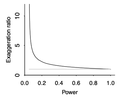
Fig 9; exaggeration ratio as a function of statistical power, for unbiased estimates that are normally distributed. When power gets much below 0.5, the exaggeration ratio becomes high (that is, statistically significant estimates tend to be much larger in magnitude, compared to true effect sizes) (Gelman & Carlin, 2014).
Another factor that may predispose effect sizes to be inflated is the presence of researcher bias. Scientists face many incentives to publish statistically significant results- this can result in decisions (made consciously or unconsciously) that predispose the data to be interpreted in a way that maximises statistical significance. For example, P-hacking refers to running a variety of statistical analyses but tending to publish the analyses that produce a significant result. Relatedly, HARKing (hypothesizing after the results are known) refers to presenting post-hoc hypotheses as if they were made prior to collecting the data. In addition, there may be political or economic motivations that motivate a research finding (e.g. drug trials that involve people with shares in companies that might go on to sell that drug).
To the best of my understanding, it is the interaction of publication bias and low power (the ‘winner’s curse’) that appears to be the most significant factor driving up Type M errors, for the RCTs we are likely to evaluate. In particular, Fanelli et al. (2017) examined a large and random sample of meta-analyses (1,910 in total) taken from all disciplines, assessing the effects of various features that have been postulated to result in bias. This was completed by testing the extent to which a set of parameters reflecting risk factors for bias were associated with a study’s likelihood to overestimate effect sizes, via metaregression. They found that small-study effects (i.e. being low-powered) were by far the largest source of bias; small-study effects explained as much as 27% of the variance in effect size, while the individual risk factors for bias (such as whether the study was run via industry) tended to account for around 1-2% of this variance.
Guidance for researchers
If you had never seen this study, what would your expectation of the effect size be for the intervention in question? (It’s probably better to have a highly speculative estimate of this rather than no estimate at all).
One way to form this expectation would be to look at the broader literature of similar interventions, to get a sense of the effect size—while using Table 1 (below) to sense-check likely effect size inflation.
Assess how well-powered the RCT is.
In general, small expected effect sizes combined with small samples are likely to be underpowered. So a behavior or attitude change experiment with a sample size of 40 is likely to be underpowered, while an experiment with thousands of people assessing changes in iron level with iron supplements is less likely to be underpowered.
Ideally, you want to get a numerical estimate of the study’s power. See guidelines here about how to do this.
Estimate the resultant effect size inflation, using figure 9 below (e.g. 20% inflation for a particular RCT). This is the lower bound for the total discount factor, since this is the effect size inflation that is occurring due to low power (not including effects from researcher bias, or poor methodological design).
Assess other likely forms of bias. For most RCTs (exception is well-powered RCTs), note that small-study effects will probably have a more significant effect upon internal reliability than these forms of bias.
Are there methodological flaws in the RCT? It can be helpful to scan Cochrane’s risk of bias guidance to get a sense of this.
Check for selection effects (was selection of individuals successfully randomised across conditions)? There may be other methodological flaws that you can spot beyond these categories.
Assess if the RCT was likely to have suffered from ‘Hawthorne effects’; where the participants in an RCT know or notice that they are under observation, and alter their behavior as a result (e.g., the recipient of a cash transfer knows that they are being observed, so deliberately spends her money on an asset that she thinks the experimenter would approve of). Adjust for this as necessary.
It may help to examine some examples of the Hawthorne effect listed here.
Estimate the extent to which you think any errors are likely to have inflated the effect that was found (e.g. 10% inflation).
Examine evidence for researcher bias.
Is the analysis pre-registered, and if so did the researchers stick to this? It will usually say in the paper if the analysis is pre-registered; e.g. CTRL-F ‘pre-register’ or ‘register’ on the paper to find the details quickly. If the researchers stuck to an analysis plan, the effect of researcher bias is likely to be smaller.
Without a pre-registered plan, is there any information that suggests to you that the researchers have chosen to analyse the study in a particular way so as to maximise the effect size/ reaching statistical significance? If so, to what extent do you think this affected the effect size? (E.g. 15% inflation).
Calculate the total discount, as 1/ the product of the individual discounts above. So here, this would be 1/ (1.2 * 1.1 * 1.15) = 0.66. This suggests that your total adjustment is 66% x [study estimate of effect size].
If there are multiple RCTs providing evidence for a given intervention:
Option 1 (quickest): use one RCT to form the estimate, and use the other RCTs to form your baseline expectation of effect size in step 1. I would recommend basing your effect size estimate upon either the RCT that is best powered, or the one that is most directly applicable to the charity/ intervention in question (so it is easier to work out the generalisability discount). If all the RCTs are underpowered (and you think it is plausible that non-significant results may not have been published), make sure that you adjust your baseline estimate accordingly by referring to Fig 9.
Option 2 (more thorough): run each RCT through steps 2-4, and average the resultant effect size.
Option 3 (more time consuming, perhaps a potential goal for the future): use formal methods to account for publication bias across multiple studies, for instance using JASP meta-analysis software. I found this paper useful to get an overview of different methods.
Is there discrepancy between your (discounted) estimate of effect size based on the RCT result, and your best-guess estimate from step 1? If so, adjust according to your credence in your step 1 estimate.
For example, in some scenarios you might place 25% weight on the step 1 estimate, and 75% weight on the discounted estimate of the effect size. The percentage split will vary according to the quality of the data used to form your step 1 estimate.
For example, some interventions will already be well-studied with multiple different RCTs. In this case, you might weight your step 1 estimate with greater credence than the effect estimate from the specific RCT that you are working from. (e.g. 80% weight on step 1 estimate, 20% on discounted estimate of effect size).
For other interventions, you might have had to produce a step 1 estimate using a different intervention type. Depending on the similarity of this intervention, this could suggest placing stronger credence in your discounted estimate of the effect size based on the RCT result.
Similarly, you might have had to produce a step 1 estimate using non-RCT evidence (e.g. observational evidence). In most cases, I would expect that you should then place stronger weight on your discounted estimate of the effect size based on the RCT result.
Alternative method; if you already have a strong sense of the likely effect size irrespective of the RCT in question, you could also use the retrodesign package to estimate effect size inflation (see the instructions for a Type S error above).
Sanity check and adjust, using Table 1 below.
| Study | Methods | Field | Discount (to get to ‘true’ effect size’) | Notes |
| Coville & Vivalt 2017 | Bayesian, retrodesign package | Development economics | 59% | Database includes a lot of very well-studied interventions (e.g. cash transfers). Database is primarily RCTs. Median power of included studies was 18-59%. |
| Open Science Collaboration, 2015 | Running replications | Psychology | 49% | Replications of 100 experimental and correlational studies in 3 well-known psychology journals. Not specific to RCTs. |
| Camerer et al. 2016 | Running replications | Economics | 66% | Replications of 18 experimental economics studies in two well-known economics journals. Includes RCTs and other designs. I am unsure why this is higher than Coville & Vivalt; I would have predicted that these replications would not replicate as well as they did. |
| Camerer et al. 2018 | Running replications | Social science (published in Science and Nature, 2010-2015) | 50% | Replications of 21 experimental social science studies that were originally published in Nature or Science. |
| Bartoš et al. 2022 | Bayesian, RoBMA | Medicine (meta-analyses) | 57% | Not peer-reviewed yet |
| Bartoš et al. 2022 | Bayesian, RoBMA | Economics (meta-analyses) | 46% | Not peer-reviewed yet |
| Bartoš et al. 2022 | Bayesian, RoBMA | Psychology (meta-analyses) | 72% | Not peer-reviewed yet- I am skeptical of this bearing in mind the results from Open Science collaboration |
Table 1; putting replication and meta-analytical estimates of effect size inflation together. This table may be better viewed on pg 16 of the google doc here.
Fig 9; exaggeration ratio as a function of statistical power, for unbiased estimates that are normally distributed. When power gets much below 0.5, the exaggeration ratio becomes high (that is, statistically significant estimates tend to be much larger in magnitude, compared to true effect sizes) (Gelman & Carlin, 2014).
Q2: What is the possibility of a Type S error?
Type S errors are when the measured effect is in the wrong direction. These errors are plausible when power is low (below around 0.2); see Fig 3. When evaluating a study, red flags for the possibility of a Type S error are (1) the intervention is not well studied (i.e. this is the first published RCT on the topic), such that there is considerable uncertainty around the effect size, (2) the RCT data is noisy, with a high standard error, (3) the RCT sample size is small, relative to the expected effect size, (4) a negative direction of effect is plausible for the metric of interest.
For example, it would make sense to check for the possibility of a Type S error for an under-powered RCT examining behavioral change in response to a new intervention. It would not make sense to check for a Type S error if there are multiple high-powered RCTs on the intervention. Overall, my best estimate is that between 0 − 15% (and likely closer to 0%) of the RCTs within our CEAs should have a Type S discount- see below for the papers that informed this estimate.
It is possible to estimate the likelihood of a Type S error by accounting for the standard error, and the likely effect size. The easiest way to do this is to use the package retrodesign() in R; this relies upon a well-validated mathematical function which is described here (Gelman & Carlin, 2014, pg 7). One difficulty of this method is the estimation of an unbiased sample size—reading the next section (about the likely magnitude of effect size inflation) may help researchers to make this estimation. I also note the existence of the Social Science Prediction Platform (developed by Prof. Vivalt)- I think it is likely that in the future we will be able to source priors about likely effect sizes from websites such as this.
Fig 3: Type S error rate as a function of statistical power, for unbiased estimates that are normally distributed. When power gets below 0.1, the Type S error rate becomes high. Taken from (Gelman & Carlin, 2014)
Guidance for researchers
Assess whether a Type S error is plausible for the RCT in question.
Is it mechanistically plausible that the direction of effect could go in the other way, and does the data appear likely to be underpowered? Remember that only around 15% of our RCTs are likely to need a Type S adjustment.
To determine whether the study is underpowered, in some cases this will be obvious from eyeballing the study. The RCT is likely to be underpowered if the data is noisy, the expected effect size is small, and the sample size is small.
As a rule of thumb, an effect size of d < 0.2 suggests the effect size is small.
If the ratio of the standard deviation to the mean is >1, this suggests that the data is noisy.
See Fig 4 to get a sense of how required sample size (to reach >80% power) varies according to effect size and the spread of the data- although note that this is for a t-test with two groups (sample size will need to be larger for more complex designs).
The paper may also state its power, or the minimum detectable effect (MDE); check the pre-registration if there is one. MDE is the minimum effect size that the test should detect, with a minimum probability (usually 80%); if the MDE is higher than your best estimate of the effect size, it is reasonably well-powered. It is also possible to calculate power yourself; see instructions here.
If you assess that there is a risk for Type S error, the best option is to assess the likelihood of this risk using the retrodesign package in R.
Install and open retrodesign. You then need to run the command retrodesign(A,B,C) where A is the expected effect size (which you estimate), B is the standard error (from RCT), and C is the statistical significance threshold (from RCT), e.g. 0.05. The $type S output will give you the expected likelihood that the RCT result is in the wrong direction. See Fig 5.
You can then use this value directly in the CEA (as a ‘X% chance this effect size went in the other direction’ for the RCT in question).
Fig 4; top row shows how sample size predicts power at different sized treatment effect, bottom row shows how sample size predicts power at different sized standard deviation. Note that this is for a simple research design (t-test with two groups, continuous outcome measure). Taken from https://egap.shinyapps.io/power-app/
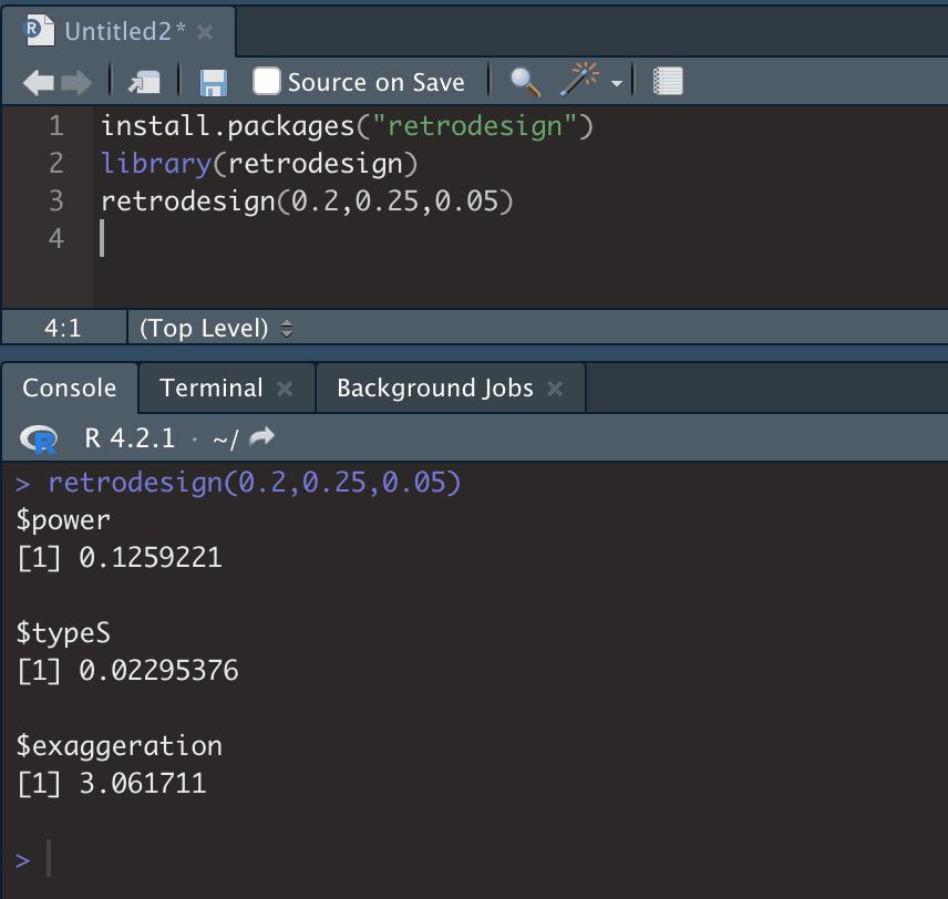
Fig 5; running retrodesign in R is very straightforward. 0.2 is the estimated effect size, 0.25 is the standard error, and 0.05 is the alpha (type 1 error). This RCT is low-powered (13% power), and there is ~2% chance of a Type S error. It is also estimated that the estimated effect size is around 3X as large as the true value, although note that this depends critically on your estimate of the true effect size.
External validity
Q3: Will RCT results generalise to a new area?
The final question to assess is whether these RCT results—which we’ve now discounted to our best estimate of the real effect, in the specific context of the RCT—will generalise to a new area. It could be the case that the effect in a new population is either larger or smaller than it was in the RCT. Clearly, most researchers will run their RCT in an area where they expect it to have a significant impact- meaning that we should expect the intervention to have a smaller effect in the new context. However, there will be exceptions to this rule. For example, if charities are able to operate in regions that are well-suited to the intervention at hand, but where RCTs are not possible.
For internal reliability, we can get quite far in our estimates by accounting for power, and looking at typical discounts suggested by meta-analytic or replication studies. Unfortunately, there is little applicable data for external validity—this means that this section is shorter. However, there are some reasons to expect that the external validity component is likely to account for more of the variability in FP recommended charities’ success than the internal reliability of the original RCTs. Note that the high internal reliability of RCTs is often contrasted with potential shortcomings in external validity (e.g.; Peters et al., 2016). In particular, Vivalt’s (2020) paper suggests that around 35% of RCTs have effects going in the other direction in different contexts, and that effect sizes differ by around 99% on average; these effects appear larger than those that we usually think about for internal reliability. However, I view these estimates as an upper-bound for the average effect; note that (since we are estimating from our discounted value), we are asking ‘given our best estimate of the true effect of the RCT, what will the effect be in a new area?’ as opposed to ‘how do the results of this RCT predict the results of a different RCT?’
I suggest estimating the degree to which an RCT result will generalise by examining the mechanism by which the intervention appears to work; do the necessary local conditions for this intervention hold in the new context? Some interventions will require more local conditions to hold than others, and therefore may have very heterogeneous effects across different areas. For example, vitamin supplementations work in a similar fashion across contexts; regions where large numbers of people lack that nutrient are therefore likely to benefit. On the other hand, behavioral or educational interventions may require lots of conditions to hold. For example, the presence of motivated teachers to carry out the intervention, presence of misconception about a particular health-related behavior, motivation to learn the new information, etc.
Duflo & Banerjee (2017) outline four key ways that RCTs may fail to generalise, which are outlined below as a method to estimate external validity. These are specific sample differences, hawthorne effects, equilibrium effects and special care effects. Sample differences refer to differences between the RCT population and the population in the new context that will affect the success of the intervention; e.g. if a population that a radio intervention plans to expand to does not have high rates of radio listenership, the intervention will likely be less effective. Hawthorne effects refer to the way in which being observed during an RCT may alter people’s patterns of behavior; e.g. obeying hand-washing instructions more often if a person is aware that they are being observed. General equilibrium effects refer to emergent effects that appear when a program is being operated at a larger scale; e.g. a cash transfer program having effects upon the local economy once enough cash transfers have been received. Finally, special care effects refer to when an intervention is implemented differently at scale relative to how it is during an RCT; e.g. a teaching intervention that is carried out less rigorously when it is scaled out to an entire teaching district.
Guidance for researchers
Examine how the study population is different from the new population
Are there different baseline rates of people who would stand to benefit from the intervention? For example, if the intervention is a vitamin supplement, and there are different rates of vitamin deficiency in this population relative to the RCT population. If so, model this out in the CEA directly (predicting ‘number of people treated’).
List out the necessary conditions for the intervention to work, and assess if they are likely to hold for the new population (and whether the new population is likely to experience smaller or larger effects from the RCT population accordingly).
For example, FEM uses radio shows to inform people about modern contraception- so more people use contraception and fewer people die from maternal mortality. In order to work in a new location, there needs to therefore be (1) unmet need for contraception, (2) a high number of people listening to the radio, (3) local contraceptive availability, (4) the presence of misinformation about contraception, (5) a relatively high maternal mortality ratio (among other conditions).
In the model, adjust for these features. For example, maternal mortality might be lower in the new locations- requiring a discount to account for this.
Note: it is entirely possible that the effect could even go in the opposite direction in the new location. Vivalt (2020) suggests that around 35% of RCTs (before accounting for these population differences) will have effects that go in the other direction. Consider what local conditions could cause this to happen, and the likelihood of these conditions.
If not already included in the ‘internal validity’ adjustment, assess for Hawthorne effects.
Assess if there are likely to be partial or general equilibrium effects, and model out if so. RCTs compare the difference between treatment and comparison populations in a given area, and are therefore unable to pick up effects which only become apparent once a program is scaled up. For example, the scale up of a cash transfer program could cause changes to a local economy.
Assess if there are likely to be ‘special care’ effects; will the intervention be conducted less well, when conducted at scale?
The Vivalt (2020) paper finds a difference of −0.081 (standardized effect size, see Fig 12) for studies that are run by the government, relative to NGOs/ academic work. I think this is likely to be capturing a special care effect.
Sanity check; look at the discounts for other interventions, and check if this seems reasonable.
A worked example
RCT effect in question: Glennerster et al. (2022) find that there is a 5.9 percentage point increase in women using modern contraception after a radio show. How will this result generalize to a new country in sub-Saharan Africa? [Note that this is a hypothetical example, that is not up to date for the specific charity that this is loosely based upon].
3.a. Internal reliability
Step 1: form a baseline estimate. I found ~16 studies with a mean effect size of 16 percentage points, but 25% of those studies found no effect. I assume that all study estimates are around 50% inflated (might seem high, but see Table 1, also note that these studies were not all RCTs) = 16 x 0.75 x 0.5 = 6 percentage point increase expectation.
Step 2: Find power of the RCT. I couldn’t find this within the paper, but this was in the pre-registration, estimated at 80%. This estimate was calculated for a 6 percentage point in power, which (as indicated from step 1) seems reasonable- I therefore used this estimate of study power.
Step 3: account for likely inflation due to the interaction of power and publication bias. Since it’s 80% powered, this effect will be small, and I estimate it at ~5% using Fig 9.
Step 4: look for evidence of researcher bias. I looked through the cochrane guidelines to check I didn’t miss anything- the main risk of bias I could see comes from potential social desirability bias in the survey data, but the administrative data (number of contraceptives purchased) supports this survey data. I estimated that this effectively increases the effect size estimate by 15% (originally estimated this at 10%, but bumped up after sanity checks below).
Step 5: Compare and adjust to baseline estimate. My total discount was 82% [1/ 1.06 x 1.15], suggesting an effect size of 4.84 [0.82 x 5.9]. In this case, I do not want to adjust my 4.92 baseline estimate; I think it is likely that I did not sufficiently discount the estimated effect sizes in this baseline estimate.
Step 6: sanity check and adjust, by checking table 1. Sanity checking here bumped up my estimate of the researcher bias. Most relevant for this study; Coville & Vivalt, 2017; Camerer et al. 2016.
My total internal reliability discount: 82%. This is still more optimistic than the table 1 results, but this study is unusually well-powered. I did not include a Type S adjustment since this study is well-powered.
3.b. External validity
Step 1: Do necessary conditions hold? I assessed various necessary conditions, including ‘presence of high unmet need for contraception’, ‘presence of lack of information/ lack of information that make women less likely to use contraception’ and ‘local contraceptive availability’ across the RCT context and new context. Overall, the conditions held- but the women in the RCT tended to be unusually close to healthcare centers (potentially making it easier for them to get contraception). I decided to discount 20% here, but I note that I still have uncertainty here.
Step 2: Were there social desirability effects in the RCT, that won’t occur when this intervention is scaled to the new area? Yes, but this was already accounted for in step 4 of the internal reliability estimate.
Step 3: Are there special care effects in the RCT, that won’t occur when intervention is scaled to new area? Potentially; radio shows might become less culturally relevant and thereby persuasive as program scales up. I discounted by 20% here but still have uncertainty.
Step 4: Will there be general equilibrium effects, that are not captured within an RCT? This is important for the nature of this intervention, and could go either way. For example, perhaps there will be spillover effects at scale, where women who did not listen to the radio show become newly aware of contraceptives, and there is some likelihood of a change in social norms. On the other hand, there is some potential for unintended negative effects at scale (e.g. if a less well-designed show is put on air and creates backlash). This is my most significant source of uncertainty- I modelled some scenarios into the CEA directly (including positive equilibrium effects), with an additional discount of 5%. I would update this if we became aware of new evidence.
Step 5: calculate the external validity discount [1/ 1.2 x 1.2 x 1.05 = 66%)
Final step: compare the internal and external validity discounts (82% and 66%) to our other discounts (a list of all current FP discounts), which here did not generate any further changes.
Conclusions
This report outlines methods to estimate the appropriate discounts that go into our CEAs, when adjusting RCT estimates of effect sizes. We should estimate the true effect size (by discounting the RCT’s estimate of the effect size by the internal reliability discount), then estimate the degree to which this effect will be observed in the context that the charity is operating in (by using the external validity adjustment). Within the context of internal reliability, I especially highlight the importance of statistical power, and its interaction with publication bias; low-powered studies (as well as producing false negatives) are likely to produce very inflated estimates of effect size. In addition, I argue that external validity is hugely important yet easy to under-appreciate, since there is little empirical work examining the degree to which RCT results generalise. The aim of this work is to make our discounts less subjective and improve accuracy, and to improve our ability to predict how well interventions will work in new areas; I think this work is likely to be most helpful for establishing discounts for ‘risky’ interventions that are comparatively less well-studied.
Bibliography
Duflo, E., & Banerjee, A. (2017). Handbook of field experiments. Elsevier.
Ellison, A. M. (2004). Bayesian inference in ecology. Ecology Letters, 7(6), 509–520.
Appendix
Notes on Relevant Papers
This section is split by the key questions (“How larger should we expect Type M errors to be?”, “What is the possibility of a Type S error?” and “Will RCT results generalise?”) and contains an overview of the key papers that I used to design these guidelines. These notes will be most relevant for readers seeking empirical evidence on these topics.
Q1: How large should we expect Type M errors to be?
Meta-assessment of bias in science, Fanelli et al. 2017
Most of the papers reviewed here were used to form estimates of the baseline rates of effect size inflation, but I include Fanelli et al. as evidence about the relative importance of different sources of bias.
Examined a large and random sample of meta-analyses (1,910 in total) taken from all disciplines, assessing the effects of various features that have been postulated to result in bias. This was completed by testing the extent to which a set of parameters reflecting risk factors for bias were associated with a study’s likelihood to overestimate effect sizes, via metaregression.
They then tested various independent variables, to test for whether they appeared to be associated with bias (see list below). Bias was assessed using meta-regression, where a second-order meta-analysis was used (weighted by inverse square of the respective standard errors), assuming random variance of effects across meta-analyses.
Size of study.
Grey literature versus journal article. Any record that could be attributed to sources other than a peer-reviewed journal was classified as grey literature; e.g. working papers, PhD theses, reports and patents.
Year of publication within meta-analysis.
Citations received.
US-study versus not.
Industry collaboration versus not.
Publication policy of country of author.
Author publication rate.
Author total number of papers, total citations, average citations, average journal impact.
Team size.
Country to author ratio,
Average distance between author addresses.
Career stage of either.
Female versus male author.
Retracted author or not (whether authors had coauthored at least one retracted paper).
Small study effects accounted for around 27% of the variance of primary outcomes, whereas gray literature bias, citation bias, decline effect, industry sponsorship, and US effect, each tested as individual predictor and not adjusted for study precision, accounted for only 1.2%, 0.5%, 0.4%, 0.2%, and 0.04% of the variance, respectively. There was some additional evidence that effect sizes were more likely to be overstated by early-career researchers, those working in smaller or long-distance collaborations, and those previously responsible for scientific misconduct. In addition, there was some evidence that US-based studies and early studies report more extreme effects, but these effects were small and hetereogeneously distributed across disciplines. Finally there was some evidence that grey literature was more likely to underestimate effects relative to peer-reviewed work (presumably due to researchers being more likely to publish results that are statistically significant)- but the effect was small.
I think there are some reasons that this study may have produced conservative estimates of biases apart from small-study effects; small-study effects are especially easy to capture and measure, and the authors mention the possibility of a modest Type 1 error here. Hence, I suspect that the size of the small-study effect (relative to other potential biases) may be somewhat overstated; nonetheless, this updated me in thinking that the most significant source of bias is likely to be small study effects.
See study description above. This study also estimated the magnitude of type M errors, using a Bayesian approach (implemented with the retrodesign package). Experts were asked for their estimates of effect size to generate priors, but the authors also used a meta-analytical approach to estimate the effect size inflation.
Relevant quote; ‘under-powered studies combined with low prior beliefs about intervention effects increase the chances that a positive result is overstated’.
Median power was estimated at between 18% − 59%.
The median exaggeration factor of significant results was estimated at 1.2 using expert predictions to form the prior. Using random-effects meta-analysis to form the prior suggested that this estimate should be 2.2.
The results around the exaggeration of effect sizes suggest that we should discount the average developmental economics study by around 59% (using the midpoint exaggeration factor of 1.7, between 1.2 and 2.2).
Estimating the Reproducibility of Psychological Science. Open Science Collaboration, 2015
This paper ran replications of 100 experimental and correlational studies published in three psychology journals, using high-powered designs (average power was estimated to be >90%).
Relevant quote; ‘low-power research designs combined with publication bias favoring positive results together produce a literature with upwardly biased effect sizes’.
The average replication effect size was 49% the size of the original study.
Evaluating replicability of laboratory experiments in economics. Camerer et al. 2016
This paper ran replications of 18 studies in well-known economics journals (American Economic Review and the Quarterly Journal of Economics) published between 2011 and 2014. These replications all had estimated statistical power > 90%.
The average replicated effect size was 66% of the original.
This paper ran replications of 21 systematically selected experimental studies in the social sciences published in Nature and Science between 2010 and 2015.
The average replicated effect size was around 50% the size of the original effect.
The authors surveyed over 26,000 meta-analyses from medicine, economics and psychology.
The medicine dataset comes from Cochrane systematic reviews, published between 1997 and 2000. The economics data comes from Ioannidis and colleagues (2017), published between 1967 and 2021. The psychology dataset comes from between 2011 and 2016 (Stanley et al., 2018). It seems plausible that differences across fields may result from the different nature of the datasets (i.e. publication years) rather than specific field differences.
True effect sizes were estimated using a publication bias and correction technique called RoBMA, that I am unfamiliar with. Since the study is not yet published (it is a pre-print) and there is no peer review/ commentary on the paper, I am unsure whether the study methods are appropriate or not. These were used to estimate the inflation factor between meta-analyses across fields, see Figs 11 and 12 below.
Fig 11; unadjusted and adjusted values from meta-analyses across medicine, economics and psychology. Y-axis indicates prior probability for effect, and secondary y-axis the Bayes factor in favor of the event (independent of the assumed prior probability of event. Black line indicates median, and light grey is the interquartile range.
Fig 12; average overestimation factor for effect sizes of meta-analyses across different fields, based on Cohen’s d and assuming presence of an effect.
The overestimation factors above suggest a discount of 57% for medicine, 46% for economics, and 72% for psychology meta-analyses effect sizes. I am surprised that psychology is lower than economics and medicine, and skeptical that this might be due to the specific datasets used across fields.
Q2: What is the possibility of a Type S error?
This paper does not provide estimates of the likely rates of Type S error across studies (my main focus in this section) but I include it for easy reference since it provides some of the mathematical foundations for calculating Type S error, and walks through examples about using the retrodesign package.
In this paper, the authors argue that we should expect most interventions to have some kind of effect—but these effects could be very small. Thus, using hypothesis testing (where we either accept or reject the possibility of a null effect) is fundamentally flawed. From this perspective, the problem is not about identifying an effect where it does not exist, but rather incorrectly estimating the effect. This can create two errors; Type S (sign) and Type M (magnitude) errors. It is possible to estimate these errors. This approach requires the researcher to (i) estimate the true underlying effect , and (ii) define a random variable drep that represents a hypothetical replication study under the exact same conditions. drep has the same standard error as the original study, centered around the mean . It is therefore possible to estimate the Type S error as the probability of the replication finding a significant effect in the opposite direction to the hypothesised true value, divided by the probability of finding a significant effect (Coville & Vivalt, 2017; Gelman & Carlin, 2014). This is coded within the retrodesign R package.
I also note this relevant quote (from page 647) ‘It is quite possible for a result to be significant at the 5% level–with a 95% confidence interval that entirely excludes zero–and for there to be a high chance, sometimes 40% or more, that this interval is on the wrong side of zero. Even sophisticated users of statistics can be unaware of this point–that the probability of a Type S error is not the same as the p value of significance level’.
The authors estimated the rate of Type S and M errors, using the methods laid out above (with the retrodesign package). They also estimated rates of false positive and false negatives, using the Bayesian framework outlined in the Ioannidis (2005) paper (see below). These were all estimated within the AidGrade database (635 studies covering 20 different types of interventions in development economics). Priors about effect size (required to estimate Type S and M errors) were generated from 125 experts.
The results (see Fig 6) suggest that the rate of Type S errors in developmental economics studies are low (around 0).
The median false positive report probability was estimated to be between 0.001 and 0.008. The false negative report probability was estimated to be between 0.512-0.624 (so the probability of false negatives is fairly high; a non-significant result may still be true).
This updates me in thinking that Type S errors may be relatively uncommon in the kinds of studies that we use (and the importance of attending to the possibility of false negatives!) However, I also note that the studies within the AidGrade database tend to be well-studied (i.e. the majority of the studies are around cash transfers). This may therefore be optimistic when applied to the kinds of interventions that we study as a whole.
Fig 6; from (Coville & Vivalt, 2017). Table shows the median power, false positive report probability, type S error and type M error via expert estimates of study impact (EE), fixed effect (FE) and random-effects (RE) meta-analysis.
Why Most Published Research Findings are False (Ioannidis 2005)
In this highly influential paper, Ioannidis uses a Bayesian framework to estimate the rate of false positive findings across modern molecular research. PPV (the post-study probability that the finding is true) is described below, where is the Type 2 error rate, is the Type 1 error rate, and R is the ratio of ‘true relationships’ to ‘no relationships’ among those tested in the field (see derivation in paper; Ioannidis, 2005);
PPV = (1-)R/(R-R + )
Adding in u as ‘the proportion of probed analyses that would not have been research findings but nevertheless end up presented as such’ (bias), generates the equation below;
PPV = ([1- ] R + uβR)/(R + α − βR + u − uα + uβR)
This suggests that relatively ‘low’ levels of bias can considerably effect PPV; see Fig 7.
Fig 7; post-study probability of true finding, at different pre-study odds and levels of bias (u). From Ioannidis et al. (2005).
An additional problem comes from the problem of having multiple research groups running similar studies; due to selective reporting, we can expect that PPV will decrease according to the number of studies being conducted which are testing the same hypothesis. For n independent studies of equal power, the 2 × 2 table is shown in Table 3: PPV = R(1 − βn)/(R + 1 − [1 − α]n − Rβn) (not considering bias).
Fig 8; post-study probability of true finding, at 80% power and different number of research groups researching the same question. From Ioannidis et al. (2005).
Using simulations according to these formulas, Ioannidis predicts that the PPV of the average study in biomedical fields are low—since most studies are underpowered, and there are a large number of teams working on similar questions. This leads him to the conclusion that most published research findings are false.
However, I note that the biomedical field in general is very different from the developmental economic one. For example, developmental economists do not run genetic association studies (which often have very low predictive power). Note that a finding from a well-conducted, adequately powered RCT starting with a 50% pre-study chance that the intervention is true is predicted (under this framework) to be correct ~85% of the time.
In addition (and while the general point that published studies are likely to have inflated effect sizes and false positives still holds) more recent analyses have generally been more optimistic. For example, Jager and Leek place the biomedical science false positive rate at around 14% rather than >50%; see full commentary (including response from Ioannidis) here.
Overall, this updated me towards thinking that (for the kind of RCTs we typically use) the chance of a false positive is somewhere between 0 − 15%; but likely below 15%.
Taking both studies together: I think that the true Type S error rate (as in, the proportion of developmental economics RCTs that we might use within a CEA) lies between 0 and 15%. I recommend only discounting for Type S error in situations where there are ‘red flags’ indicating the potential for this type of error (where negative effect is plausible, there is little existing evidence for the intervention beyond the RCT in question, the RCT has very low power; see Guidance for Researchers above for rules-of-thumb).
Q3: Will RCT results generalise to a new area?
How much can we generalize from impact evaluations? Vivalt, 2020
This paper uses the AidGrade dataset, that comprises 20 types of interventions, such as conditional cash transfers and deworming programs. These estimates are used to estimate the degree to which the effect size estimated in one paper predict the effect size estimate from another paper (within the same intervention type).
Key findings:
Using Bayesian ‘leave one out’ analysis predicts the correct sign 61% of the time, across all studies (65% for RCTs specifically).
Adding in the best-fitting explanatory variable (turning model into a mixed model) explained ~20% of this variance.
Some evidence that studies with smaller ‘causal chain’ have smaller heterogeneity.
The median absolute amount by which a predicted effect size differs from the true value given in the next study is 99%. In standardized values, the average absolute value of the error is 0.18, compared to an average effect size of 0.12.
Quoting from an interview with Prof. Vivalt in 80,000 hours; ‘so, colloquially, if you say that your naive prediction was X, well, it could easily be 0 or 2*X — that’s how badly this estimate was off on average. In fact it’s as likely to be outside the range of between 0 and 2x, as inside it.’
Fig 12; from Vivalt (2020). Regression of standardised effect size upon study characteristics.
Other relevant sources, that did not clearly fit into Type S/ Type M framework
Two related blog articles: ‘Is it fair to say that most social programmes don’t work?’ (80000 Hours blog) and ‘Proven programs are the exception, not the rule’ (GiveWell Blog)
I place these articles together since they rely upon similar estimates. In 2008, David Anderson (assistant director at the Coalition for Evidence-Based Policy) estimated on GiveWell’s blog that ~75% of programs that are rigorously evaluated produce small or no effects, and in some cases negative effects.
In the 80,000 hours blog, David clarifies that this estimate (which has become a widely-quoted estimate in the effective altruism community) is rough, but is based on his organisation’s review of hundreds of RCTs across various areas of social policy. I note that these RCTs appear to be generally based in the US, and are of social programs; one possibility is that these programs have lower replicability than the typical programs we could fund.
I could not find data putting together the effect sizes that the Coalition for Evidence-Based Policy has typically found. In this report, they do link to some RCT studies; for example, the finding that ~90% of the RCTs commissioned by the Institute of Education Sciences since 2002 have been found to have weak or no effects.
In the 80,000 hours blog, Prof. Vivalt was then asked for her perspective upon the number of RCTs that produce significant results. She used the AidGrade data to find that around 60-70% of the intervention-outcomes that were studied within this database have insignificant meta-analysis results (when restricting attention to important outcomes). However, one caveat is that the AidGrade data contains only interventions for which there is a considerable amount of data—it may be the case that researchers are less likely to study interventions that they think might fail.
Assuming that around 60-75% of RCTs do indeed fail, what does this imply for generalisability? Broadly, I think that we should assume (for interventions that look promising, but are not backed by RCT/ strong quasi-experimental evidence) that there is a 60-75% chance that they do not work (or at least, produce sufficiently small effect sizes that a typical RCT will not identify the effect). For generalisability, I suspect that the number of RCTs that work (dependent upon another RCT studying the same intervention that has found a positive result) is higher.
Application to quasi-experimental work
Quasi-experimental work also seeks to establish a cause-and-effect relationship between an independent and dependent variable, but does not rely upon random assignment; subjects are assigned to groups based on non-random criteria. For some interventions, running an RCT is ethical or otherwise impossible, meaning that we must rely upon quasi-experimental evidence.
My current understanding (I have not done a deep dive, and am somewhat uncertain here) is that effect sizes tend to be similar across RCTs and high-quality quasi-experiments, suggesting that we do not need an additional discount merely for using a quasi-experiment rather than an RCT—but we should attend to markers of quasi-experimental methodological quality. For example, Chaplin et al. (2018) tested the internal reliability of regression discontinuity designs (primarily economics studies) via comparison with RCTs. The authors did not find evidence for systematic bias within the regression discontinuity designs relative to the RCTs. Another study ran a meta-analysis and systematic review of quasi-experimental results for socioeconomic interventions in LMIC, comparing the results to RCT estimates of effect sizes. Again, the authors did not find evidence that the quasi-experimental estimates differed systematically from the RCT estimates (Waddington et al., 2022).
Therefore, I think that working out discounts for quasi-experimental work should be almost the same as that for RCTs—but with an additional step at the beginning to assess whether the experimental designs met the necessary assumptions for causality. If methodological assumptions are not met, then we should place little to no weight on the study results, since we cannot be sure that the effect is causal from the intervention.
Here are some key assumptions to check for different quasi-experimental designs (Liu et al., 2021). Note that this is not an exhaustive list; also see here. This work is incomplete, and could deserve a full report of its own, depending on how much we rely on quasi-experimental data in the future.
For instrumental variables analysis: in IV analysis, the goal is to identify observable variables (instruments) that affect the system only through their influence on the treatment of interest X.
Are there confounding variables that influence both the instrument and the outcome?
Does the instrument influence the outcome through any way other than their effect upon treatment? E.g. imagine a scientist wanting to study the effect of exercise on wellbeing, who plans to use temperature as an instrument on the amount of exercise individuals get. However, temperature might influence mental health outside of exercise, for example through seasonal affective disorder- making it an unsuitable instrument here.
How strongly correlated is the instrument and the treatment of interest? Weak correlations may lack the power to detect the effect.
For regression discontinuity: in RDDs, the treatment of interest is assigned according to a cutoff of a continous running variable R (such as age or a standardised test score). Because the cutoff is sharp (e.g. getting an A or B grade at the margin) the treatment assignment X is quasi-random for individuals near the cutoff, allowing for the estimation of the causal effect of the treatment on the outcome.
Is there a precise cut-off, determining the treatment at that margin?
Another assumption is that individuals cannot perfectly manipulate the running variable (i.e. if some students were precisely controlling their test score so that they scrape an A without additional workload).
About Founders Pledge
Founders Pledge is a global nonprofit empowering entrepreneurs to do the most good possible with their charitable giving. We equip members with everything needed to maximize their impact, from evidence-led research and advice on the world’s most pressing problems, to comprehensive infrastructure for global grant-making, alongside opportunities to learn and connect. To date, they have pledged over $10 billion and donated more than $850 million globally. We’re grateful to be funded by our members and other generous donors. founderspledge.com
NB: The Unjournal commissioned two expert evaluations of this work: see the full reports and ratings here.
From the first evaluation abstract (anonymous):
From the second evaluation abstract (by Max Maier):
I’d love to know if this work is being used or followed up on.
This is excellent. It will definitely inform the way I work with RCTs from now on.
I would just like to quibble your use of the word “discount”. In most of the post you use it synonymously with “multiplier” (ie. a 60% discount to account for publication bias means you would multiply the experimental result by 0.6). However in your final worked example under External Validity you apply “discounts” of 20%, 20% and 5% for necessary conditions, special care effects and general equilibrium effects respectively, with the calculation 100/(100+20+20+5)*100% = 74%. This alternative definition took me some time to get my head around.
I’d also expect to see the 20%, 20%, 5% combined as multipliers, since these effects act independently: 1/(1.2*1.2*1.05) *100% = 66% (although I realise the final result isn’t too different in this case).
Thanks Stan! This is really helpful- agreed with you that they should be combined as multipliers rather than added together (I’ve now edited accordingly). I’m still mulling a bit over whether using the word ‘discount’ or ‘adjustment’ or something else might help improve clarity.
Really useful, Rosie! Could only skim (as I’m about to board a flight) but looking forward to digging deeper into this.
Thank you Joel! Hope that you had a nice flight.