The Nucleic Acid Observatory (NAO) project produced this report to guide our research on disease surveillance methods capable of detecting novel stealth pathogens. We think this report will also be useful outside the NAO, so we are sharing it more widely.

This report was written by Will Bradshaw, with detailed feedback and visualizations provided by Simon Grimm.

I. Summary

The NAO’s fundamental mission is to ensure that humanity can reliably detect stealth pandemics^[1] as soon as possible. To achieve this, we need to implement a monitoring system capable of reliably detecting novel outbreaks even in the absence of a strong clinical signal. Such a system could be based on a wide range of possible sampling strategies, including both those that collect material from individuals (individual sampling) and those that collect it from the human environment (environmental sampling). Different sampling strategies differ in key properties, including detection capability, cost, and credibility to those with the power to initiate an effective response to detection.

The detection capability of a sampling strategy depends on both the size and composition of its catchment (the population of individuals contributing material to the sample) and the microbial composition of the resulting samples. How these affect detection depends in turn on the methods used to analyze the resulting sequencing data, which can be divided into static detection (which detect potential threats based on nucleic-acid sequence features) and dynamic detection (which detect potential threats based on suspicious temporal patterns of sequence abundance). Dynamic detection methods are typically more vulnerable to noise arising from temporal variability in catchment and microbial composition, and hence benefit more from large, consistent catchments and stable microbial communities with high pathogen abundance.

Major costs associated with biosurveillance include those associated with gaining and maintaining approval; sample collection; sample processing; metagenomic sequencing; and computational analysis. The cost of a given sampling strategy will depend in many ways on its scale, in terms of the size of the catchment sampled; the geographic area covered; the temporal density of sampling; and the degree of sequencing effort. In general, individual sampling approaches will exhibit a steeper increase in costs as scale increases, due to the need to collect and process rapidly increasing numbers of individual samples. Conversely, environmental sampling approaches will typically exhibit flatter financial and personnel costs with increasing scale, at the cost of decreasing per-person sensitivity. Environmental sampling strategies also seem likely to incur substantially lower regulatory burdens than individual strategies that involve collecting and handling individually identifiable medical information.

Finally, in addition to detection capability and cost, sampling strategies differ in their ability to enable and motivate an effective response to a novel outbreak. In general, sampling strategies with smaller catchments will provide more actionable information to policymakers when it comes to targeted responses (e.g. contact tracing and isolation). Sampling strategies that provide identifiable cases and affected constituencies may also prove more effective at motivating a response from policymakers with strong political incentives to avoid drastic interventions. However, sampling strategies that might struggle to enable and motivate an immediate targeted response can still provide scientists and policymakers with invaluable situational awareness about pathogen distribution, prevalence and spread. Overall, a multi-tiered approach, in which large-catchment surveillance triggers more targeted monitoring when signs of an outbreak are found, may prove most effective at balancing competing needs for sensitivity, credibility, and cost-effectiveness.

I. Introduction & background

To reliably detect stealth pandemics^[1], we need a suitable monitoring system that collects samples in the right places, processes them in the right way, and analyzes the resulting data using algorithms with the right detection capabilities. So far, the work of the NAO has primarily focused on wastewater sampling. This has many advantages, but also faces major challenges in the context of untargeted pathogen detection. Thus, while we will continue to invest in wastewater sampling, we also want to make sure that we aren’t missing out on alternative, possibly more effective strategies. This report provides an introduction and conceptual framework for this work.

Goals & assumptions

In order to prioritize among different sampling approaches, we need to be clear about what our goals are. There are several key assumptions going into this analysis that it’s important to make explicit:

Initial detection of a stealth pandemic: The core objective of the NAO is to detect novel stealth biothreats – pathogens that are able to infect many people without being detected by existing systems of infectious disease surveillance^[2], e.g. due to a very long incubation period. This goal is very different from ongoing monitoring of a known threat: the objective is to detect the pathogen & identify it as a major threat at least once, anywhere. Techniques and approaches that are suitable for ongoing monitoring may not be appropriate for effective initial detection, and vice versa^[3].
Detection, not suppression: In traditional public health, the primary function of early detection of outbreaks is to suppress them via targeted interventions (e.g. isolation, contact tracing, or ring vaccination). Many discussions of biosurveillance tacitly assume this framing. We are both more pessimistic and more optimistic than this traditional framing: pessimistic that a stealth threat will be detected early enough to achieve suppression, and optimistic that even much later detection (e.g. at 1/1000 or even ¹⁄₁₀₀ cumulative incidence) can provide major benefits^[4]compared to no detection. As such, we are not primarily assessing detection strategies on their ability to enable rapid targeted response or suppression, but rather on their ability to enable reliable early detection per se.
Pathogen-agnostic detection via metagenomic sequencing: When it comes to initial detection of a novel pathogen, targeted detection approaches like qPCR are inadequate; instead, we need an approach that is capable of picking up signatures of pathogens we aren’t already looking for. Currently, the most promising technology for this purpose is metagenomic sequencing (MGS)^[5] (Gauthier et al., 2023). While it’s possible that a future NAO-like system may come to rely on technologies other than MGS, for the purpose of this report we’re assuming that MGS is the core detection technology being used.

Categorizing sampling approaches

Given our focus on human-infecting pathogens, all our sampling strategies of interest involve collecting material produced by human bodies. This material can be collected directly from individuals (individual sampling) or from environmental substrates into which it has been shed (environmental sampling^[6]). Individual and environmental sampling thus represent two broad categories, each of which encapsulates a number of specific sampling strategies. Examples of promising individual sampling strategies include saliva, blood, and combined nose/throat swabs, while examples of promising environmental strategies include municipal wastewater, aggregated airplane lavatory waste, and air sampling from airplanes or crowded indoor areas.

**Figure 1: Environmental vs individual sampling.** Individual sampling collects specimens (e.g. swabs, blood, saliva) directly from individual people, whereas environmental sampling collects environmental specimens (e.g. from air, wastewater, surfaces) containing emitted human material.

Within both individual and environmental sampling, strategies can differ in both the type of material that is collected (specimen type), and the population of individuals contributing to the sample (catchment). Both have critical implications for the value of a given sampling strategy, and are discussed further below.

Formalizing threat detection methods

The suitability of different sampling approaches for early detection of a subtle pathogen depends on the computational method used to analyze the resulting data. As such, it’s helpful to have a clearer formalization of how such methods might function.

Consider a population of human individuals, within which we aim to detect any newly-emerged stealth pathogen as early as possible (within resource constraints). Call this the population of interest; depending on context, this could be the population of the world, a particular country, or a specific sub-population^[7].

In order to detect pathogens spreading in the population of interest, we collect samples containing material contributed by some subset of individuals from that population; this contributing subpopulation is the catchment. These samples are subject to sample preparation, MGS, and data processing; the end result is a collection of nucleic-acid sequences (e.g. k-mers or contigs) along with counts assigned to each sequence quantifying their abundance in the sample.

From here, the goal is to identify sequences corresponding to genuine threats: pathogens (especially stealth pathogens) present in the catchment that threaten the health of the population of interest. To do this, the sequences and counts are fed into one or more threat detection methods that attempt to distinguish threatening from non-threatening sequences^[8]. While a thorough survey of possible detection methods is beyond the scope of this report, we can sketch out two broad categories that share certain features:

Static detection methods focus primarily on the sequence component of the processed data, attempting to identify nucleic-acid sequence features associated with potential threats. Potential forms of static detection include:

Homology-based detection, wherein sequences are tagged as threatening based on their similarity to existing known threats (e.g. a novel sarbecovirus or filovirus).
Genetic engineering detection, wherein detection algorithms identify signatures of artificial sequence tampering as signals of a potential threat.
Pathogenicity prediction, wherein detection algorithms attempt to directly identify sequence features predictive of causing ill-health.
Heuristic by-eye approaches, wherein abundant sequences in a sample are manually inspected for “obvious” warning signs (which might include elements of any or all of the above approaches).

Dynamic detection methods, in contrast, focus on the observed counts of different sequences over time, identifying potential threats based on specific temporal patterns that are deemed suspicious. Potential forms of dynamic detection include:

Growth-based detection, wherein the counts associated with particular sequences are used to estimate (explicitly or implicitly^[9]) the true abundance of the corresponding sequence in the population at large. Aggregating these estimates over time (and, in some cases, space^[10]) and applying statistical inference to the resulting time series, these methods aim to identify growth signatures that are indicative of a potential threat (Consortium, 2021).
Novelty detection, wherein sequence data from a given sampling strategy (e.g. at a specific sample collection site) is collected over time to establish a baseline, and novel sequences appearing for the first time are subsequently flagged as suspicious.

**Figure 2: Examples of dynamic vs static detection methods.** Homology-based detection tags viruses based on their similarity to known threats (e.g., H5N1 influenza). Genetic engineering detection identifies signatures of artificial sequence tampering. Growth-based detection uses sequence count time-series data to track and flag suspicious growth patterns. Novelty detection uses previously seen sequencing data as a reference against which to identify and flag novel sequences.

Static and dynamic detection methods have some important differences:

Agnosticity/generality: Any static-detection method must make specific assumptions about what characteristics make a sequence potentially threatening. They thus leave open the risk of missing threats that do not satisfy (or have been deliberately engineered to evade) these assumptions. In contrast, dynamic detection approaches only assume that a pathogen’s sequence will grow in a particular way, which seems much more difficult to avoid or evade.
Specificity: The very minimality of their assumptions may also leave dynamic-detection approaches more vulnerable to false positives: sequences that happen to grow in a “threatening” manner without posing a true threat to the population of interest. Conversely, the reliance of static methods on more detailed features of NA sequences will likely allow for fewer false positives (i.e. greater specificity).
Reliance on time-series data: By definition, dynamic detection methods identify threats by tracking changes in sequence abundance over time. As a result, this approach requires collecting relatively dense (and expensive) MGS time series, in which the relative abundance of each sequence can be estimated at multiple successive time points. In contrast, static methods can identify threats based on data from a single time-point, and so do not require extensive time-series data^[11].
Reliance on accurate abundance estimates: As described above, some dynamic detection methods rely on the ability to discern particular growth signatures over time. To achieve this, growth trends inferred from sequencing data should correspond to real epidemiological trends in the population of interest. These methods will fail if noise and (inconsistent) bias in the data obscure these real-world trends. In static detection or novelty detection, conversely, the accuracy of inferred abundances relative to the real population is not of critical importance, as long as (1) the sequence of interest occurs at all in the dataset, and (2) its count is high enough to be confident that it reflects a real sequence present in the catchment (as opposed to a sequencing error, contamination, etc)^[12].

Many detection methods – especially those that are heuristic in nature – will in practice combine elements of both temporal and static detection, and consequently sit at an intermediate point on these various axes. Ultimately, the detection of a threat is a Bayesian process, in which many different features of a sequence (both temporal and static) can contribute to an overall assessment of threat.

III. Detection capability across sampling strategies

Central to any discussion of the viability of any sampling strategy is its detection capability: its ability, when implemented competently and combined with a suitable detection method, to identify a wide range of threats in a reliable and timely manner. The detection capability of a sampling strategy is affected by a range of factors, most of which fall into two broad categories: those pertaining to the catchment of individuals sampled by a given strategy, and those pertaining to the composition of the specimen obtained^[13].

Catchment

As defined above, the catchment of a sampling strategy is the set of human individuals contributing material to the collected sample^[14]. This catchment is a subset of the population of interest, within which we are aiming to detect the emergence of a novel pandemic pathogen. The relationship between the catchment and the population of interest – in particular, the size of the catchment and its composition relative to the population of interest – is a central factor in the overall efficacy of any given sampling approach.

Catchment size

In accordance with the law of large numbers, aggregated samples taken from catchments of increasing size will tend in composition towards the overall composition of the population of interest, reducing the expected deviation between the measured abundance of each sequence in sequencing data and its true prevalence in the larger population. For dynamic detection methods, this effect is highly desirable, as it reduces noise in estimates of sequence abundance and increases the power of these methods to detect suspicious temporal trends. As a result, catchment size is a key factor to consider when selecting a sampling strategy for dynamic detection.

In many cases, larger catchments are also desirable for static detection methods. When the prevalence of the pathogen of interest is sufficiently high in the population, the reduced noise of larger catchments enables these methods to detect it more reliably. However, when prevalence is low, larger catchments can actually harm detection capability for these methods: in this latter case, a large-catchment sample will fall below the method’s detection threshold with high probability, while a small-catchment sample that contains a few infected individuals might exceed the threshold through chance alone (Figure 6, Appendix 1). Hence, while frequently helpful, increased catchment size is less of an unalloyed good for static than for dynamic detection.

Large catchments also have other potential downsides in practice:

Most obviously, for many (but not all) sampling approaches, sampling from a larger catchment is much more expensive than sampling from a small one.
Sampling from a larger catchment will also generally increase the background complexity of the sample, as different individuals will contribute distinct microbial signatures to the final dataset.
For some sampling approaches such as wastewater, increasing catchment size also frequently increases the degree of dilution by abiotic or nonhuman material, reducing pathogen abundance.

Small catchments allow creation of richer metadata on the individuals included in the catchment, enabling both richer data analysis and more targeted responses.

In some cases, the tradeoffs between small and large catchments can be avoided by taking many small-catchment samples in parallel, then pooling material or data from these samples to create larger catchments synthetically. This allows the effective catchment to be adjusted as desired, while retaining the rich metadata of the small-catchment samples. However, for sampling approaches with relatively flat cost/catchment scaling (such as wastewater), this parallel pooled approach will often still be much more expensive than sampling a smaller number of larger catchments.

Geographic bias

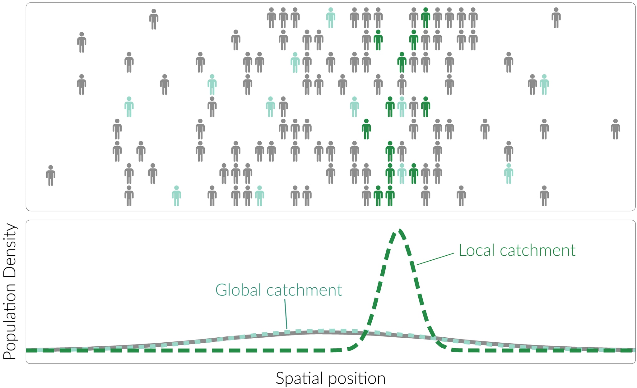
In any monitoring system, the population of interest will be distributed spatially across some area^[15] – for example, the US or the world. Different catchments will vary in how representatively they reflect this geographic distribution; we can define a catchment as more global if its spatial distribution is representative of the population of interest, and more local if it instead exhibits a strong bias towards particular locations.

Any sampling method requires geographical co-location between the sampling mechanism and the sample source, be that a person or an environmental area. As a result, many sampling strategies^[16] are constrained to sample local catchments, composed primarily of people who live and/or work close to the sampling location. In order to instead achieve global sampling, some special effort is needed, such as:

Conducting local sampling in parallel at multiple locales (e.g. wastewater sampling at multiple treatment plants in different cities). This method is simple and effective, but resource-intensive and logistically challenging.
Conducting remote sampling, in which individuals widely distributed in space are requested to collect and mail samples in their local area (e.g. self-collected swabs or “citizen science” surface swabbing (McDonald et al., 2018; Roberts, 2020)). This approach is potentially lower cost than parallel local sampling, but requires coordination among many unaffiliated individuals.
Targeting local sampling to sites that are highly enriched for individuals who have recently traveled long distances, effectively achieving a more global catchment at a single sampling site. The most attractive sites for this purpose will typically be long-distance transport hubs and/or vehicles, with airports and airplanes offering the greatest potential for a truly global sample. While cost-effective, the catchment sizes accessible with this approach will inevitably be lower than some more local sampling approaches – for example, the population contributing the airport wastewater, while more geographically diverse, will also be much smaller than that contributing to the local wastewater treatment plant.

The effect of the geographic bias of a catchment on detection capability is significantly more complex and case-dependent than that of catchment size. In particular, the impact of spatial distribution on detection depends heavily on the dynamics of disease spread relative to the spatial migration of individuals. For example, if the incidence of new infections is sufficiently low relative to migration, then the issue of local versus global sampling can largely be ignored, as the disease will effectively be well-mixed across the population even at low prevalence. Conversely, if migration is very slow relative to disease spread, then the disease will progress as a series of largely independent outbreaks in different locations, in which case the location at which sampling is taking place will have a major impact on the speed of detection. Intermediate cases will exhibit complex interdependencies between transmission, migration and other factors, the understanding of which will require further investigation.

**Figure 3: Geographic bias.** Catchments can differ in their spatial representativeness compared to the population of interest (gray). A more global catchment (blue) is more representative of the spatial distribution of the underlying population, while a more local catchment (green) exhibits unrepresentative concentration in one or more particular areas.

Consistency of composition

Some sampling methods will sample from a very consistent population: the residents of a particular building, the students and staff at a particular school, the employees of a particular company. Others will show some variation in catchment from day to day, but maintain a reasonably high level of consistency overall: the current population of a particular town, or the commuters passing through a particular rail station at 8.45am.

Other sampling strategies, however, will sample from catchments that change dramatically from day to day. Long-distance travel hubs especially will often show very low consistency, with only a minority of the population^[17] passing through on day n returning on day n+1. Furthermore, the distribution of geographic origins of these individuals might also vary significantly day to day; given that the metagenomic content of both human and environmental samples shows significant geography-dependent variation, this could result in greatly increased day-to-day volatility in the resulting MGS data.

As with local vs global catchment distribution, we don’t yet have a deep understanding of the effects of catchment inconsistency on detection capability. On the one hand, as an additional source of noise and variable bias, it could act as a confounding variable reducing the detection capability of dynamic detection approaches^[18]. On the other hand, by varying the catchment day-by-day, it can avoid risks of “lock-in” to a poorly chosen initial catchment, thus increasing the detection capability of static detection methods. Further investigation is needed to improve our understanding of the importance of this factor in assessing different sampling strategies.

Correlation with infection status

When it comes to outbreaks, not all catchments are created equal. Some groups – whether delineated by location, occupation, or some other factor – will tend to experience more infections earlier in an outbreak than the general population. Early in an outbreak, these groups (e.g., healthcare workers, airline staff, military personnel, or international travelers) will be significantly enriched for infected individuals – e.g. because they are especially likely to contact infected individuals, be targeted by a bioattack, or be particularly susceptible to infection.

Targeted sampling of such “sentinel” populations could thus give advance warning of an outbreak. Weighed against this benefit, the main costs of focusing on a sentinel population are (1) the logistical burden associated with identifying and targeting members of that population, and (2) the smaller catchment size associated with excluding non-members from your sample. The severity of (1) depends on the sentinel population in question; populations that are easier to identify and access will make more promising sentinels than those that are more difficult. The severity of (2) depends substantially on the cost/catchment scaling of your chosen sampling approach: the cheaper a marginal increase in catchment size, the greater the counterfactual cost of focusing on a smaller sentinel group compared to the general population.

At a finer level of detail, some populations will be enriched for cases at a particular stage in the course of infection, e.g. disproportionately early or late cases. The most obvious example of this is symptomatic patients at a hospital: while these will be highly enriched for diseases able to cause their symptoms, they will also be highly enriched for being in the later, symptomatic stages of infection. As a result, relying on hospital cases might result in later detection than if you’d sampled a population with a greater proportion of early cases, even if the total enrichment for cases is much lower (e.g. municipal wastewater).

Specimen composition

Even holding the catchment constant, different sampling strategies will provide specimens with significantly different microbial content. MGS data produced from these specimens will thus differ in both the observed abundance of pathogens of interest, and in the composition and complexity of the microbial background. Both of these can have important implications for our ability to detect novel threats.

Pathogen abundance

Not all pathogens get everywhere in the human body. They have tropisms, disproportionately infecting specific cell and tissue types within the host and avoiding others. Respiratory pathogens will tend to infect cells or tissues in the respiratory tract, while gastrointestinal pathogens will tend to be found at high concentrations in the gut lumen and gut epithelial cells. Pathogens also differ in the breadth of their tropism, with some (e.g., SARS-CoV-2) infecting many more cell types than others (e.g., influenza)(Flerlage et al., 2021). As a result, different pathogens will show dramatically different shedding patterns, which in turn result in very different abundances across different sampling strategies, whether individual (e.g., nasal swabs vs blood samples) or environmental (e.g., wastewater vs air sampling).

In addition to shedding dynamics, pathogen abundance in a sample will also be critically affected by its physical stability during the period between shedding and sample collection. This is especially important for environmental sampling: the more quickly a pathogen degrades in the environment – whether due to environmental nucleases, abiotic reactions, bacteria, bleach, or some other factor – the less of it will be detectable in the sample upon collection. In addition to the composition of the environment (e.g. concentration and activity of nucleases), stability depends heavily on the physical composition of the pathogen in question: for example, enveloped viruses will generally be less stable outside a host than non-enveloped viruses, and RNA genomes will degrade more quickly than DNA genomes.

In addition to physical stability, the locational/spatial stability of the pathogen at the sampling site will also affect its abundance. If some process (e.g. water flow or cleaning) removes intact pathogen from the sampling location before it can be sampled, its measured abundance will be reduced. Higher rates of removal effectively act as degradation processes, reducing the half-life of the pathogen at the sampling site.

Finally, the abundance of a pathogen in an environmental sample will depend on the degree of dilution of human material in the sample by nonhuman and/or abiotic material. This again varies dramatically between sample types – for example, municipal wastewater is far more dilute (with many more liters of water per unit mass of stool) than airplane wastewater, and virtually all environmental sampling will be far more dilute than any kind of human sampling. Increased dilution has the effect of reducing the absolute abundance of all human-originating microorganisms in the sample, as well as potentially introducing new, non-human-infecting microorganisms (e.g. from soil or other animals).

Factors like these are primarily of concern insofar as they alter the relative abundance of pathogen sequences compared to other nucleic acids in the sample. Lower relative abundance will increase noise and reduce sensitivity, necessitating a corresponding increase in sequencing effort (& concomitant costs) to compensate. Variability in relative abundance (absent true changes in pathogen prevalence) will confound dynamic detection methods by obscuring trends in pathogen growth. Within reason, changes in absolute pathogen abundance that do not affect relative abundance (e.g. due to dilution by abiotic material) are not of huge concern for detection capability; however, extreme reductions in absolute abundance, beyond our ability to concentrate the sample, can impact sensitivity^[19].

While some processes affecting pathogen abundance (e.g. flow rates) can to some degree be considered in isolation from any specific pathogen, others (e.g. physical stability or tropism) depend sensitively on the specific properties of the pathogen in question. While we can make some general statements about the classes of pathogens we’re concerned about from the perspective of a severe pandemic^[20], it’s difficult to make strong claims ex ante about the detailed shedding or stability characteristics of the pathogens a system needs to detect. Consequently, it’s important to design these systems with a broad range of pathogen properties in mind.

Microbial background

In addition to the abundance of the pathogen itself, the abundance and composition of a sample’s microbial background^[21] also impacts detection capability. Different sampling strategies will result in backgrounds that differ dramatically in both composition and complexity: the microbiome of stool is very different from that of exhaled breath, which in turn is very different from that of saliva. MGS data obtained from these different samples will in turn exhibit very different composition.

The most straightforward way in which background affects detection capability is by altering the relative abundance of any pathogens of interest in the sample. Due to the compositional nature of sequencing data, the number of reads obtained from any given sequence depends not only on the abundance of that sequence, but also on that of all other sequences in the sample. A sample with lower absolute pathogen abundance might still produce a stronger signal if the absolute abundance of the microbial background is lower still.

Beyond simple considerations of relative abundance, many people have the intuition that more complex samples – those whose background is more taxonomically diverse and/or shows more complex temporal dynamics – should be worse for detection capability. Formalizing this is challenging, but there are a number of factors that point in the direction of this intuition being roughly correct. In discussing these, we can broadly separate arguments that relate to the static taxonomic diversity of the background from those that relate to dynamic changes in composition over time.

**Figure 4: Static complexity and Dynamic complexity.** Static complexity refers to the taxonomic diversity of an individual sample, with more complex samples containing more taxa and/or more uneven abundance distributions among taxa. Dynamic complexity refers to changes in composition over time, with highly dynamic samples demonstrating larger abundance shifts and the frequent appearance and disappearance of species.

Static complexity: Microbial communities, whether real or synthetic, can differ dramatically in the number and relative abundance of microbial taxa they contain. We expect some sample types of interest (e.g. wastewater) to be much more complex than others (e.g. blood^[22]), with implications for their suitability for threat detection:

One way to increase the relative abundance of pathogens of interest, and thus increase sensitivity, is to specifically reduce the absolute abundance of the background. This kind of background depletion is much more effective when the background is simpler: by depleting only one or a few particular taxa, one can significantly alter the relative abundance of any potential pathogens of interest. For example, in the case of human sampling, targeted removal of human nucleic acids can significantly increase MGS sensitivity & reduce costs (Shi et al., 2022). Conversely, when the background is highly taxonomically complex (comprising e.g. many hundreds or thousands of abundant taxa), background depletion becomes much more challenging.
The more taxonomically complex the background, the more difficult it will be to characterize its composition adequately to reliably detect notable/threatening additions. From a Bayesian perspective, observing a new sequence in a highly simple and stable community is a strong signal of a genuine & interesting addition, while in a highly complex community with many low-abundance members it is much more likely to be an artifact of measurement or random low-level fluctuations.
Depending on the distribution of abundances within a microbial community, high taxonomic complexity can confound attempts to improve detection capabilities through increasing sequencing effort. If a community is roughly power-law distributed, with very many low-abundance species, increasing sequencing effort will roughly always discover previously unseen (but not genuinely new) taxa, while measurement noise will constantly raise “new” taxa above the threshold of detection. As such, complex communities will likely exhibit much more severe problems with noise and false positives than simple ones.

Dynamic complexity: No microbial community is static. Over time, the microbial composition of a series of specimens taken from a given source will change as a result of endogenous ecological and evolutionary processes; seasonal and other changes in the abiotic environment; changes in the composition of the sample catchment; and changes (e.g. dietary) in the behavior of the human individuals in that catchment. The composition of any resulting metagenomic dataset will thus vary over time, with several important effects on detection capability:

Changes in background will directly affect the measured abundance of any pathogen of interest, both by altering its relative abundance in the sample and by altering the average sequencing efficiency (McLaren, Willis and Callahan, 2019) of the background relative to the pathogen. The resulting noise might obscure true changes in pathogen abundance. Dynamic detection methods will be especially vulnerable to these effects, increasing the relative attractiveness of static approaches for high-temporal-complexity samples.
Growth and decay of non-pathogenic background taxa will also increase the number of innocuous sequences that appear to be undergoing threatening changes in abundance, resulting in an increased number of false positives raised by any given dynamic detection method. This effect will be particularly strong in cases where the rate of growth seen in background fluctuations is similar to the typical growth rate expected in genuinely concerning cases. If severe enough, this effect could impede a system’s ability to effectively investigate and identify true threats.
Finally, high dynamic complexity will also further confound attempts to improve sensitivity through background depletion (see above), as the most important background components to deplete will change over time.

IV. Cost

So far, we’ve discussed the detection capabilities of different sampling strategies in the abstract, without reference to the cost and feasibility of actually implementing different approaches. However, given limited resources, the costs associated with any given sampling strategy – in money, time, personnel hours, political capital, and other resources – are inevitably critical in determining its viability.

Any sequencing-based biosurveillance project will incur a wide range of different costs, both fixed and scaling with the number of sites, samples, and days of operation (Table 1). These costs will vary substantially between sampling approaches, both in their initial magnitude and their scaling behavior. While a detailed, quantitative cost model of different sampling strategies would require in-depth modeling beyond the scope of this report, we do feel able to make some qualitative observations:

Stage	Description	Examples	Scaling
Approval	Delays, staff time, and possibly payments involved in securing agreement from site owners, regulatory authorities, and other major stakeholders.	Approval from hospital to collect samples from patients; approval from airport operator to install samplers in terminals.	Primarily per-site.
Sample collection	Space, equipment, consumables, staff time and energy costs involved in obtaining samples from individuals or the environment.	Buying and operating a wastewater autosampler; collection tubes for saliva samples; staff training for collection of nasal swabs.	Per-site (space, equipment), per-sample^[23] (consumables), and per-unit-time (staff pay, equipment rental).
Sample processing	Costs associated with laboratory processing of collected samples, including lab space, equipment, consumables, and staff time.	Rental of lab space & equipment; reagents for sequencing library prep; operation of freezers for long-term sample storage; staff time for protocol development and execution.	Per-site (if performed locally but not if centralized), per-sample (consumables), per-unit-time (staff pay, equipment rental)
Sequencing	Costs associated with sequencing processed samples, including relevant consumables, equipment, energy costs, and staff time.	Costs of purchasing & operating sequencers; payments to outsource sequencing to external providers.	Per-site (if performed locally but not if centralized), per-sample (consumables, outsourcing costs), per-unit-time (staff pay, equipment rental).

Table 1: Cost categories associated with each sampling strategy.

Sampling effort: In general, most individual sampling approaches seem likely to be markedly more intensive than environmental sampling in terms of materials (especially consumables) and staff time. The number of “sample collection operations” performed by each staff member per day is likely to be much higher for individual^[24] than environmental sampling, as is the number of parallel laboratory steps carried out during sample processing.
Pathogen abundance: In contrast, the relative abundance of a pathogen of interest will likely be considerably higher in a well-chosen individual sample from an infected individual, than in an environmental sample. This means that the amount of sequencing required could be significantly lower, reducing costs commensurately.
Costs of catchment scaling: Individual and environmental sampling also differ significantly in the costs associated with increasing catchment size. To a first approximation, the cost of individual sampling scales linearly with catchment size: in order to sample twice as many people, one needs roughly twice as many consumables, twice as much staff time, et cetera^[25]. In contrast, for environmental sampling, one can often alter catchment size without increasing sampling effort by changing the sampling location, resulting in flat or even decreasing cost as catchment size increases^[26]. Consequently, very large catchments can become extremely expensive for individual sampling, but are far more feasible for environmental sampling approaches.
Costs of spatial scaling: The cost of obtaining a more global sample also differs between sampling strategies. Individual samples that can be self-collected with high success rates (e.g. saliva) are far more amenable to cheap distributed sampling approaches than those that require trained medical staff (e.g. blood). Adding a well-located major airport to a wastewater sampling program will have a far bigger effect on spatial coverage than adding a new wastewater treatment plant.
Regulatory overhead: Many individual sampling approaches generate individually identifiable information that may be subject to complex and onerous medical privacy laws in many jurisdictions. Conversely, environmental sampling collects human material in a highly aggregated and anonymized fashion, to which there appear to be relatively few legal barriers in the United States. While the details of regulatory approval in different jurisdictions lie beyond the expertise of the current authors, it seems likely that establishing and maintaining such approval will often be significantly more costly for individual than for environmental sampling.

V: Credibility and response

In addition to cost and detection capability, one final important way in which sampling strategies differ is in their capacity to trigger an effective response to prevent or mitigate a severe pandemic. This varies along two main axes: the degree to which that sample provides the information necessary to enable different kinds of response actions, and the degree to which threat detection in a sample represents a credible signal that can persuade relevant authorities to take such actions.

When it comes to enabling effective response, a key factor is the degree of detail available regarding the infected individuals giving rise to the pathogen signal^[27], which is typically a function of catchment size. Small-catchment samples can provide a great deal of detailed information about the infected individuals, up to and including their identity, and are consequently far more useful for targeted responses such as isolation, contact tracing, and follow-up testing. In contrast, large-catchment samples (e.g. municipal wastewater) only enable broad responses, such as an increase in surveillance effort or (in extreme cases) a local lockdown. Intermediate catchment sizes enable intermediate responses – for example, identification of a threat in wastewater from an individual plane would narrow the field of potential cases to that plane’s passengers and crew.

This difference in response capability is sometimes raised as a major disadvantage of large-catchment sampling strategies; however, as discussed above, targeted response is not a central concern for the NAO, and as such is not a primary consideration in this report.

A second, more subtle link between sampling strategy and response is the degree to which threat detection in a given sample type is credible to the actors (e.g. governments, pharmaceutical companies, or the medical & scientific establishment) that have the ability to execute relevant interventions. If nobody listens when a threat is identified, then the system that identifies it is useless. If certain sampling strategies (most plausibly, clinical sampling) are much more credible to these actors than others, it might be necessary to deploy them even if they are otherwise uncompetitive with alternative approaches. The cost of this could be mitigated by rolling out these credible approaches in response to an initial detection event elsewhere, at some cost in speed.

VI: Conclusion

In this report, we reviewed a number of key factors affecting the relative attractiveness of different sampling strategies for a biosurveillance system focused on early detection of novel stealth pandemics. These factors include the composition and size of a strategy’s catchment; the microbial composition of the resulting samples; the cost of scaling that strategy in different ways; and the ability of the resulting data to motivate a meaningful response. Along the way, we have defined and clarified terminology describing different sampling strategies, detection methods, and pathogen properties of relevance for comparing sampling approaches.

Future work will build on the qualitative frameworks described here to create more sophisticated quantitative models investigating different factors – including a more thorough and quantitative treatment of the cost of different sampling strategies – as well as applying these frameworks to concretely evaluate specific sampling strategies of interest.

Acknowledgments

While this report was written by the named authors, the ideas expressed are the product of several years of thinking about the problem of early detection by a number of people. We’d like to especially thank Kevin Esvelt, Mike McLaren, Jeff Kaufman, Dan Rice, Charlie Whittaker, & Lenni Justen for their thoughtful comments, suggestions and contributions before and throughout the writing process.

Appendix 1 - The impact of sample size on static detection sensitivity

The following defines a simple toy model to explore how probability of detection of a novel pathogen varies with catchment size. It assumes a simple, uniform model of infection and shedding; a simple, static, MGS-based detection method with a flat detection threshold measured in number of pathogen reads; and uniform sampling across the catchment with no bias based on infection status. The code for Figures 5 to 7 is available here.

1. Defining the model—number of pathogen reads

Consider a population of interest $P$ in which a pathogen of interest is spreading. Currently, a fraction $p$ of your population is positive for the pathogen in a way which can be detected with metagenomic sequencing^[28]. You select $n$ individuals at random from $P$ to form your catchment, $C$ . The number of infected individuals in $C$ is given by $K \sim B i n o m i a l (n, p)$

Each individual in $C$ contributes equal nucleic acid to your sample. In addition, some amount of nucleic acid is contributed by non-human sources, depending on the sample type: this nonhuman fraction is equal to the amount contributed by $z$ individuals. The fraction of input nucleic acid from each individual is therefore given by $\frac{1}{n + z}$ , and that from the nonhuman fraction by $\frac{z}{n + z}$ .

Assume that the pathogen makes up a fraction $f$ of nucleic acid from infected individuals, and none of the nucleic acid from uninfected individuals or the nonhuman fraction. For a given value of $K$ , the total fraction of nucleic acid in your sample coming from the pathogen is thus given by:

$F_{k} = \frac{f k}{n + z}$

If we sequence $r$ total reads from the pooled sample, then for a given value of $K$ , the number of reads we acquire from the pathogen is given by $R_{k} \sim P o i s s o n (λ_{k})$ , where $λ_{k} = r F_{k} = \frac{r f k}{n + z}$ .

Under this framework, the expected number of pathogen reads is given as follows:

$\begin{matrix} E (R) & = \sum k E (R | K = k) P (K = k) = \sum k \frac{r f k}{n + z} P (K = k) = \frac{r f}{n + z} E (K) = \frac{r f n p}{n + z} \end{matrix}$

We can calculate the variance in the number of pathogen reads using the law of total variance:

$\begin{matrix} V a r (R) & = E (V a r (R | K)) + V a r (E (R | K)) = E (λ_{k}) + V a r (λ_{k}) = E (\frac{r f K}{n + z}) + V a r (\frac{r f K}{n + z}) = \frac{r f}{n + z} E (K) + {(\frac{r f}{n + z})}^{2} V a r (K) = \frac{r f n p}{n + z} + \frac{r f n p}{n + z} \frac{r f (1 - p)}{n + z} = E (R) [1 + \frac{r f (1 - p)}{n + z}] \end{matrix}$

If the sample is purely human in composition (i.e. $z = 0$ ) these equations simplify to:

$E (R) = r f p$

$V a r (R) = E (R) [1 + \frac{r f (1 - p)}{n}]$

Hence, when the non-human component of the system is negligible, the average number of pathogen reads is independent of catchment size, while the variance in pathogen reads declines with increasing catchment size. At very large catchment sizes, the variance is equal to the mean, and $R$ exhibits Poisson-like behaviour with a rate parameter of $r f p$ .

2. Defining the model—probability of detection

Let us assume that we are applying some static detection method to the dataset with a simple integer read threshold of $T$ : when $R > T$ , we are able to correctly identify the pathogen as a threat with high confidence; otherwise, we cannot. Given some value of $K$ , The probability of correctly identifying the threat is therefore given by:

$Q_{k} = P r (R > T | K = k) = 1 - P r (R \leq T | K = k) = 1 - e^{- λ_{k}} \sum_{j = 0}^{T} \frac{λ_{k}^{j}}{j!}$

The overall probability of identification is then given by the expectation of $Q_{k}$ over $K$ :

$Q = \sum_{k = 0}^{n} Q_{k} \times P r (K = k) = \sum_{k = 0}^{n} [1 - e^{- λ_{k}} \sum_{j = 0}^{T} \frac{λ_{k}^{j}}{j!}] [\frac{n!}{k! (n - k)!} p^{k} (1 - p)^{n - k}]$

When $n$ is large and $z$ is small, $1 - Q$ tends towards the cumulative Poisson probability with $λ = r f p$ :

$A = {lim}_{n \to \infty} Q = 1 - e^{- r f p} \sum_{j = 0}^{T} \frac{(r f p)^{j}}{j!}$

3. Example results

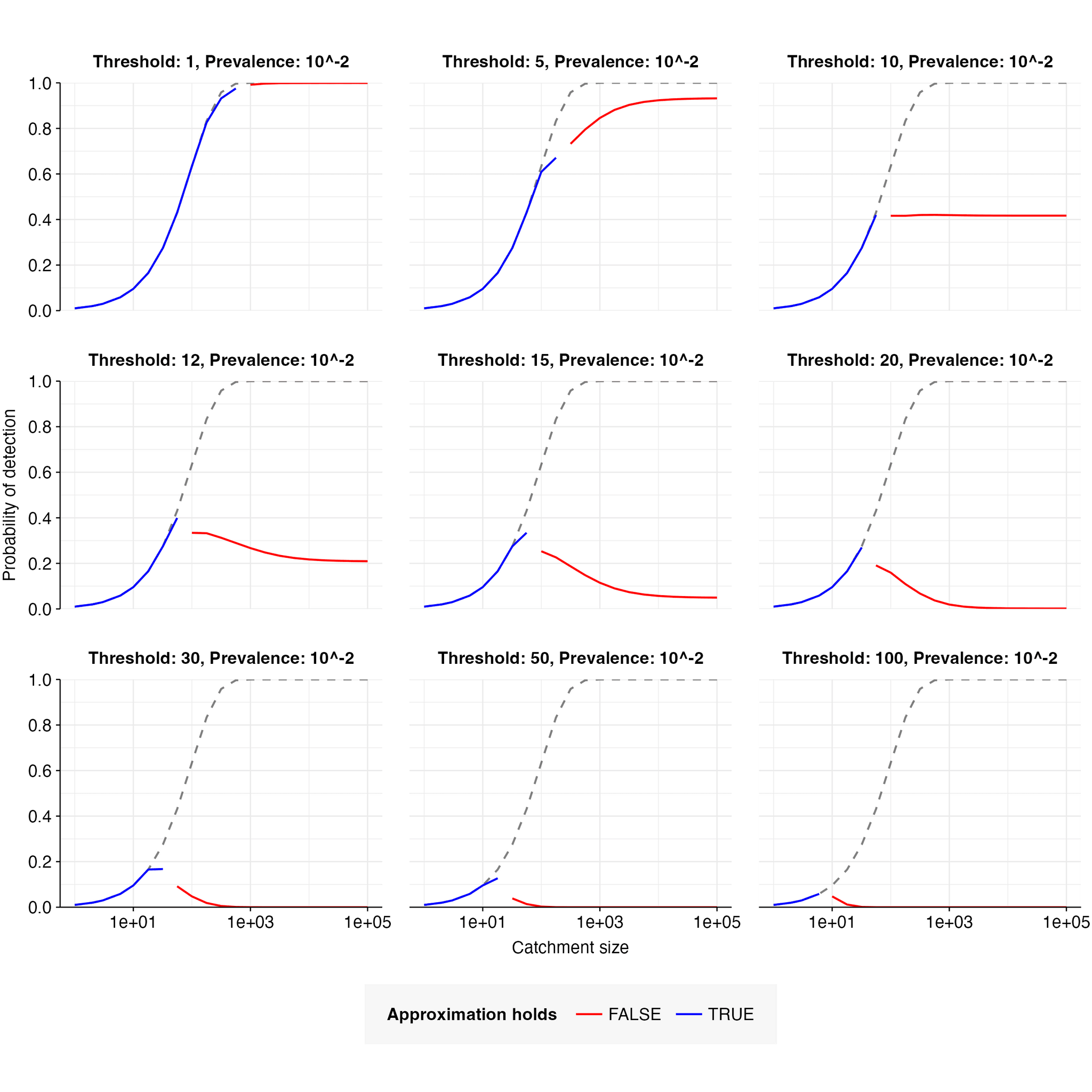
For this example case, let $z = 0$ (no non-human fraction), $f = 10^{- 6}$ , and $r = 10^{9}$ . Given these parameters, $F_{k} = 10^{- 6} \frac{k}{n}$ , $λ_{k} = 10^{3} \frac{k}{n}$ , $E (R) = 10^{3} p$ . The probability of detection $Q$ can then be calculated for a range of catchment sizes, prevalence values, and detection thresholds (Figures 5 & 6).

**Figure 5:** Probability of detection for a range of catchment sizes, prevalences, and detection thresholds, given the specified parameter values. Horizontal dashed lines indicate the asymptotic detection probability $A$ predicted previously.

**Figure 6:** Probability of detection for a range of catchment sizes and detection thresholds, given a prevalence of 1% and the parameter values previously specified . Horizontal dashed lines indicate the asymptotic detection probability $A$ predicted previously.

When $E (R) \geq T$ , $Q$ increases monotonically with catchment size, converging toward $A$ as the catchment becomes sufficiently large; $A \approx 1$ when $E (R) >> T$ , but shrinks as $E (R)$ moves closer in value to $T$ . When $E (R) < T$ , $Q$ initially increases with catchment size, but then reaches a peak and declines toward a low value of $A$ as catchment size increases further; the closer $E (R)$ is to $T$ , the higher the peak.

When the catchment is small, a single infected individual can be sufficient to cause detection; this is expected to be the case when $T$ is smaller than the expected number of pathogen reads from one person, i.e. when $T < \frac{f r}{n}$ . When this is the case, the detection probability is well-approximated by the probability of at least one infected person in the catchment, i.e. $Q \approx 1 - (1 - p)^{n}$ . This is illustrated in Figure 7.

**Figure 7**: Probability of detection for a range of catchment sizes and detection thresholds, given a prevalence of 1% and the parameter values previously specified. Gray dashed curves indicate the probability of detection predicted by a simple geometric approximation that holds when a single infected individual in the catchment is expected to cause detection. Solid lines indicate the actual probability of detection, with blue indicating regions where the approximation is expected to hold and red indicating where it is not.

References

Consortium (2021) ‘A Global Nucleic Acid Observatory for Biodefense and Planetary Health’, arXiv:2108.02678 [q-bio] [Preprint]. Available at: http://arxiv.org/abs/2108.02678 (Accessed: 23 October 2021).

Flerlage, T. et al. (2021) ‘Influenza virus and SARS-CoV-2: pathogenesis and host responses in the respiratory tract’, Nature reviews. Microbiology, 19(7), pp. 425–441. Available at: https://doi.org/10.1038/s41579-021-00542-7.

Gauthier, N.P.G. et al. (2023) ‘Agnostic Sequencing for Detection of Viral Pathogens’, Clinical microbiology reviews, 36(1), p. e0011922. Available at: https://doi.org/10.1128/cmr.00119-22.

McDonald, D. et al. (2018) ‘American Gut: an Open Platform for Citizen Science Microbiome Research’, mSystems, 3(3). Available at: https://doi.org/10.1128/mSystems.00031-18.

McLaren, M.R., Willis, A.D. and Callahan, B.J. (2019) ‘Consistent and correctable bias in metagenomic sequencing experiments’, eLife. Edited by P. Turnbaugh et al., 8, p. e46923. Available at: https://doi.org/10.7554/eLife.46923.

Roberts, A.P. (2020) ‘Swab and Send: a citizen science, antibiotic discovery project’, Future science OA, 6(6), p. FSO477. Available at: https://doi.org/10.2144/fsoa-2020-0053.

Shi, Y. et al. (2022) ‘Metagenomic Sequencing for Microbial DNA in Human Samples: Emerging Technological Advances’, International journal of molecular sciences, 23(4). Available at: https://doi.org/10.3390/ijms23042181.

Smolinski, M.S., Crawley, A.W. and Olsen, J.M. (2017) ‘Finding Outbreaks Faster’, Health security, 15(2), pp. 215–220. Available at: https://doi.org/10.1089/hs.2016.0069.

^
A stealth pandemic is one with the potential to spread very widely before being noticed or responded to. In the context of human pandemics, this primarily means a pathogen that is able to infect very many people without being detected by conventional clinical surveillance, e.g. due to a very long incubation period.
^
While some specific diseases are the subject of ongoing monitoring, systematic monitoring for new infectious diseases is generally quite limited, and reliant on the traditional “astute physician” method of initial detection (Smolinski, Crawley and Olsen, 2017).
^
The ability to efficiently transition from initial detection to ongoing monitoring will be key to the efficacy of an NAO-like system, but is not the focus of this report.
^
For example, by enabling widespread deployment of infection-mitigation measures (e.g. PPE or isolation) to protect uninfected individuals, alongside development of countermeasures that might otherwise be delayed by many months or years.
^
Two potential alternatives to MGS that have been discussed in the context of pathogen-agnostic surveillance are (1) the development of large overlapping panels of semi-specific probes targeting e.g. sequences conserved across viral families, and (2) surveillance of host biomarkers of disease via e.g. untargeted serology. While potentially promising, these approaches face their own significant technical hurdles, and are beyond the scope of this report.
^
A note on terminology. The term “environmental sampling” can be ambiguous, as it is sometimes used to refer to collecting nucleic acids from the natural environment (e.g. soil or natural watercourses). In this case, we are using it to refer to any sampling process targeting human surroundings (e.g. wastewater or buildings) as opposed to the humans themselves.
^
For example, a national government might be principally interested in detecting anything spreading in its own domestic population, while an impartial altruist or international public health body might aim to detect anything spreading anywhere in the world.
^
Once a threat has been identified, it can be subjected to a range of downstream responses, including enhanced monitoring (e.g. widespread targeted monitoring of the identified sequences), public health interventions (e.g. lockdowns or isolation of infected individuals), and intensive scientific study.
^
As an extreme example of a dynamic detection method that implicitly estimates abundances, consider an algorithm that flags if the raw count of a sequence increases by some percentage from day to day. This doesn’t make any explicit estimate of the true abundance, but the signal is only interesting because it implies the abundance is increasing.
^
For example, emergence and growth of the same sequence at multiple sites could provide important additional evidence for a threat.
^
Though even for static detection, being able to demonstrate that the sequence is present across multiple time-points could be important for validating a finding and stimulating response.
^
As a result, many sources of noise and bias in counts data are of reduced concern for static detection compared to dynamic approaches, as long as they do not cause the sequences of interest to be missed entirely or fall below the threshold of confident identification. Conversely, dynamic algorithms can benefit greatly from changes in sampling strategy that reduce the degree of noise and (inconsistent) bias in these abundance estimates relative to the population of interest.
^
Not included here are factors affecting the cost of different strategies, or their ability to motivate an effective response independently of their detection capability – these will be discussed in section 5.
^
Note that in this report, the catchment constitutes the set of individuals who actually contribute material to the sample, not those who might potentially contribute. For example, in the case of airplane wastewater, passengers who travel on a plane but don’t use the bathroom would not form part of the catchment by this definition. An alternative definition of catchment that includes potential contributors could also be a reasonable target of analysis, but is not our focus here.
^
In many cases, the population of interest is synonymous with the population occurring in some area (e.g. the US or the world). However, even POIs defined in other ways (e.g. military personnel) will still exhibit some spatial distribution.
^
Examples of sampling strategies that are unavoidably local include municipal wastewater, air sampling in residential or commercial settings, and most human sampling based on individuals visiting or passing by a particular location (such as a hospital, urban testing center, or shopping mall).
^
In the case of airports, the consistent population will primarily be made up of resident airport staff, as well as potentially some flight crews manning short-haul flights.
^
It also excludes detection methods reliant on tracking infection status in specific individuals over time.
^
At the extreme, if absolute abundance is so low that no copies of the pathogen genome are found in a sample, then no amount of concentration will rescue sensitivity.
^
E.g. respiratory pathogens seem particularly concerning.
^
We can define the background of an MGS sample as the collection of all nucleic acids not originating from a pathogen of interest. Common major components of MGS background include host material, commensal bacteria, and bacteriophages.
^
In general, individual samples are strongly dominated by human nucleic acids, resulting in lower diversity than environmental samples. Blood in particular, while not strictly sterile, lacks a resident microbiome of any significant complexity.
^
Note that, in this case, material obtained from multiple individuals that is then pooled before processing would count as a single “sample”.
^
The additional costs associated with individual sampling can be somewhat mitigated through participant self-sampling and pooling samples prior to lab processing, but these may come with other associated costs in the form of reduced sample quality and detection capability.
^
The costs of conducting individual sampling at scale can be somewhat mitigated by taking advantage of economies of scale, as well as by pooling sample aliquots prior to processing or sequencing. Nevertheless, the broad point holds that very large catchments are frequently prohibitively expensive for individual sampling approaches.
^
This is particularly apparent in the case of municipal wastewater sampling, where, depending on its location, the same autosampler sampling the same amount of material can have a catchment of a single building, a cluster of buildings, a neighborhood, or an entire city. Due to pre-existing infrastructure and expertise, it is often easier and cheaper to collect samples from a treatment plant covering an entire region than from a smaller area accessible via manhole.
^
A second relevant factor might be the amount of information available about the pathogen, for example the ability to obtain a complete genome or culture the pathogen in vitro.
^
This model thus treats infection as a binary state which is consistent across all infected individuals. In reality, of course, the strength of the metagenomic signal will vary both among infected individuals and across the time course of each infection.

Comparing sampling strategies for early detection of stealth biothreats