Summary: This post documents research by SatisfIA, an ongoing project on non-maximizing, “aspiration-based” designs for AI agents that fulfill goals specified by constraints (“aspirations”) rather than maximizing an objective function. We aim to contribute to AI safety by exploring design approaches and their software implementations that we believe might be promising, but neglected or novel. Our approach is roughly related to, but largely complementary to, concepts like Decision Transformers, Active Inference, Quantilization and Satisficing (or soft optimization in general).

It’s divided into two parts, the informal introduction and the formal introduction.

First, the informal introduction describes the motivation for the research, our working hypotheses, and our theoretical framework. It does not contain results and can safely be skipped if you want to get directly into the actual research.

Second, the formal introduction presents the simplest form of the type of aspiration-based algorithms we study. We do this for a simple form of aspiration-type goals: making the expectation of some variable equal to some given target value.^[1]

At the end of the post we give an overview of the projects status (we’re looking for collaborators!) and have a small glossary of terms.

This post is the summary for an emerging sequence on LessWrong and the Alignment Forum, authored by us and other members of the SatisfIA project team. If you wish to learn more about our approach you can read the full sequence there.

🄸🄽🄵🄾🅁🄼🄰🄻 🄸🄽🅃🅁🄾🄳🅄🄲🅃🄸🄾🄽

Motivation

We share a general concern regarding the trajectory of Artificial General Intelligence (AGI) development, particularly the risks associated with creating AGI agents designed to maximize objective functions. We have two main concerns:

AGI development might be inevitable

The development of AGI seems inevitable due to its immense potential economic, military, and scientific value. This inevitability is driven by:

Economic and military incentives: The prospect of gaining significant advantages in efficiency, capability, and strategic power makes the pursuit of AGI highly attractive to both private and state actors.
Scientific curiosity: The inherent human drive to understand and replicate intelligence propels the advancement of AGI research.

It might be impossible to implement an objective function the maximization of which would be safe

The conventional view on A(G)I agents (see, e.g., Wikipedia) is that they should aim to maximize some function of the state or trajectory of the world, often called a “utility function”, sometimes also called a “welfare function”. It tacitly assumes that there is such an objective function that can adequately make the AGI behave in a moral way. However, this assumption faces several significant challenges:

Moral ambiguity: The notion that a universally acceptable, safe utility function exists is highly speculative. Given the philosophical debates surrounding moral cognitivism and moral realism and similar debates in welfare economics, it is possible that there are no universally agreeable moral truths, casting doubt on the existence of a utility function that encapsulates all relevant ethical considerations.
Historical track-record: Humanity’s long-standing struggle to define and agree upon universal values or ethical standards raises skepticism about our capacity to discover or construct a comprehensive utility function that safely governs AGI behavior (Outer Alignment) in time.
Formal specification and Tractability: Even if a theoretically safe and comprehensive utility function could be conceptualized, the challenges of formalizing such a function into a computable and tractable form are immense. This includes the difficulty of accurately capturing complex human values and ethical considerations in a format that can be interpreted and tractably evaluated by an AGI.
Inner Alignment and Verification: Even if such a tractable formal specification of the utility function has been written down, it might not be possible to make sure it is actually followed by the AGI because the specification might be extremely complicated and computationally intractable to verify that the agent’s behavior complies with it. The latter is also related to Explainability.

Given these concerns, the implication is clear: AI safety research should spend considerably more effort on identifying and developing AGI designs that do not rely on the maximization of an objective function. Given our impression that currently not enough researchers pursue this, we chose to work on it, complementing existing work on what some people call “mild” or “soft optimization”, such as Quantilization or Bayesian utility meta-modeling. In contrast to the latter approaches, which are still based on the notion of a “(proxy) utility function”, we explore the apparently mostly neglected design alternative that avoids the very concept of a utility function altogether.^[2] The closest existing aspiration-based design we know of is Decision Transformer, which is inherently a learning approach. To complement this, we focus on a planning approach.

Working hypotheses

We use the following working hypotheses during the project, which we ask the reader to adopt as hypothetical premises while reading our text (you don’t need to believe them, just assume them to see what might follow from them).

1: We should not allow the maximization of any function of the state or trajectory of the world

Following the motivation described above, our primary hypothesis posits that it must not be allowed that an AGI aims to maximize any form of objective function that evaluates the state or trajectory of the world. (This does not necessarily rule out that the agent employs any type of optimization of any objective function as part of its decision making, as long as that function is not only a function of the state or trajectory of the world. For example, we might allow some form of constrained maximization of entropy or minimization of free energy or the like, which are functions of a probabilistic policy rather than of the state of the world.)

2: The core decision algorithm must be hard-coded

The 2nd hypothesis is that to keep an AGI from aiming to maximize some utility function, the AGI agent must use a decision algorithm to pick actions or plans on the basis of the available information, and that decision algorithm must be hard-coded and cannot be allowed to emerge as a byproduct of some form of learning or training process. This premise seeks to ensure that the foundational principles guiding the agent’s decision making are known in advance and have verifiable (ideally even provable) properties. This is similar to the “safe by design” paradigm and implies a modular design where decision making and knowledge representation are kept separate. In particular, it rules out monolithic architectures (like using only a single transformer or other large neural network that represents a policy, and a corresponding learning algorithm).

3: We should focus on model-based planning first and only consider learning later

Although in reality, an AGI agent will never have a perfect model of the world and hence also needs some learning algorithm(s) to improve its imperfect understanding of the world on the basis of incoming data, our 3rd hypothesis is that for the design of the decision algorithm, it is helpful to hypothetically assume in the beginning that the agent already possesses a fixed, sufficiently good probabilistic world model that can predict the consequences of possible courses of action, so that the decision algorithm can choose actions or plans on the basis of these predictions. The rationale is that this “model-based planning” framework is simpler and mathematically more convenient to work with and allows us to address the fundamental design issues that arise even without learning, before addressing additional issues related to learning. (see also Project history)

4: There are useful generic, abstract safety criteria largely unrelated to concrete human values

We hypothesize the existence of generic and abstract safety criteria that can enhance AGI safety in a broad range of scenarios. These criteria focus on structural and behavioral aspects of the agent’s interaction with the world, largely independent of the specific semantics or contextual details of actions and states and mostly unrelated to concrete human values. Examples include the level of randomization in decision-making, the degree of change introduced into the environment, the novelty of behaviors, and the agent’s capacity to drastically alter world states. Such criteria are envisaged as broadly enhancing safety, very roughly analogous to guidelines such as caution, modesty, patience, neutrality, awareness, and humility, without assuming a one-to-one correspondence to the latter.

5: One can and should provide certain guarantees on performance and behavior

We assume it is possible to offer concrete guarantees concerning certain aspects of the AGI’s performance and behavior. By adhering to the outlined hypotheses and safety criteria, our aim is to develop AGI systems that exhibit behaviour that is in some essential respects predictable and controlled, reducing risk while fulfilling their intended functions within safety constraints.

6: Algorithms should be designed with tractability in mind, ideally employing Bellman-style recursive formulas

Because the number of possible policies grows exponentially fast with the number of possible states, any algorithm that requires scanning a considerable portion of the policy space (like, e.g., “naive” quantilization over full policies would) soon becomes intractable in complex environments. In optimal control theory, this problem is solved by exploiting certain mathematical features of expected values that allow to make decisions sequentially and compute the relevant quantities (V- and Q-values) in an efficient recursive way using the Hamilton–Jacobi–Bellman equation. Based on our preliminary results, we hypothesize that a very similar recursive approach is possible in our aspiration-based framework in order to keep our algorithms tractable in complex environments.

Theoretical framework

Agent-environment interface. Our theoretical framework and methodological tools draw inspiration from established paradigms in artificial intelligence (AI), aiming to construct a robust understanding of how agents interact with their environment and make decisions. At the core of our approach is the standard agent–environment interface, a concept that we later elaborate through standard models like (Partially Observed) Markov Decision Processes. For now, we consider agents as entirely separate from the environment — an abstraction that simplifies early discussions, though we acknowledge that the study of agents which are a part of their environment is an essential extension for future exploration.

Simple modular design. To be able to analyse decision-making more clearly, we assume a modular architecture that divides the agent into two main components: the world model and the decision algorithm. The world model represents the agent’s understanding and representation of its environment. It encompasses everything the agent knows or predicts about the environment, including how it believes the environment responds to its actions. The decision algorithm, on the other hand, is the mechanism through which the agent selects actions and plans based on its world model and set goals. It evaluates potential actions and their predicted outcomes to choose courses of action that appear safe and aligned with its aspirations.

Studying a modular setup can also be justified by the fact that some leading figures in AI push for modular designs even though current LLM-based systems are not yet modular in this way.

Information theory. For formalizing generic safety criteria, we mostly employ an information theoretic approach, using the mathematically very convenient central concept of Shannon entropy (unconditional, conditional, mutual, directed, etc.) and derived concepts (e.g., channel capacity). This also allows us to compare and combine our findings with approaches based on the free energy principle and active inference. where goals are formulated as desired probability distributions of observations.

High-level structure of studied decision algorithms

The decision algorithms we currently study have the following high-level structure:

The agent accepts tasks given as aspirations, i.e., as constraints on the probability distribution of certain task-relevant evaluation metrics. The aspiration will be updated over time in response to achievements, good or bad luck, and other observations.
Whenever the agent must decide what the next action is, it performs a number of steps.
1. First, it uses its world model to estimate what evolutions of the evaluation metrics are still possible from the current state on, and after taking each possible action in the current state. This defines the state’s and all possible actions’ “feasibility sets”.
2. It then compares each possible action’s feasibility set with its current aspiration and decides whether it would have to adjust its aspiration if it were to take that action, and how to adjust its aspiration in that case. This defines all possible actions’ “action-aspirations”.
3. It also evaluates all possible actions using one or more safety and performance criteria and picks a combination of one or more candidate actions that appear rather safe.
4. It then randomizes between these candidate actions in a certain way.
5. Based on the next observation, it updates its beliefs about the current state.
6. Finally, in particular when the environment is partially unpredictable and the agent has had some form of good or bad luck, it potentially adjusts its aspiration again (“aspiration propagation”).

Depending on the type of aspiration, the details can be designed so that the algorithm comes with certain guarantees about the fulfillment of the goal.

🄵🄾🅁🄼🄰🄻 🄸🄽🅃🅁🄾🄳🅄🄲🅃🄸🄾🄽

Assumptions

In line with the working hypotheses, we assume more specifically the following in this post:

The agent is a general-purpose AI system that is given a potentially long sequence of tasks, one by one, which it does not know in advance. Most aspects of what we discuss focus on the current task only, but some aspects relate to the fact that there will be further, unknown tasks later (e.g., the question of how much power the agent shall aim to retain at the end of the task).
It possesses an overall world model that represents a good enough general understanding of how the world works.
Whenever the agent is given a task, an episode begins and its overall world model provides it with a (potentially much simpler) task-specific world model that represents everything that is relevant for the time period until the agent gets a different task or is deactivated, and that can be used to predict the potentially stochastic consequences of taking certain actions in certain world states.
That task-specific world model has the form of a (fully observed) Markov Decision Process (MDP) that however does not contain a reward function $R$ but instead contains what we call an evaluation function related to the task (see 2nd to next bullet point).
As a consequence of a state transition, i.e., of taking a certain action $a$ in a certain state $s$ and finding itself in a certain successor state $s^{'}$ , a certain task-relevant evaluation metric changes by some amount. Importantly, we do not assume that the evaluation metric inherently encodes things of which more is better. E.g., the evaluation metric could be global mean temperature, client’s body mass, x coordinate of the agent’s right thumb, etc. We call the step-wise change in the evaluation metric the received Delta in that time step, denoted $δ$ . We call its cumulative sum over all time steps of the episode the Total, denoted $τ$ . Formally, Delta and Total play a similar role for our aspiration-based approach as the concepts of “reward” and “return” play for maximization-based approaches. The crucial difference is that our agent is not tasked to maximize Total (since the evaluation metric does not have the interpretation of “more is better”) but to aim for some specific value of the Total.
The evaluation function contained in the MDP specifies the expected value of $δ$ for all possible transitions: $E δ (s, a, s^{'})$ .

First challenge: guaranteeing the fulfillment of expectation-type goals

The challenge in this post is to design a decision algorithm for tasks where the agent’s goal is to make the expected (!) Total equal (!) a certain value $E \in R$ which we call the aspiration value. This is a crucial difference from a “satisficing” approach that would aim to make expected Total at least as large as $E$ and would thus still be happy to maximize Total. Later we consider other types of tasks, both less restrictive ones (including those related to satisficing) and more specific ones that also care about other aspects of the resulting distribution of Total or states.

It turns out that we can guarantee the fulfillment of this type of goal under some weak conditions!

Notice that a special case of such expectation-type goals is making sure that the probability of reaching a certain set of acceptable terminal states equals a certain value, because we can simply assume that each such acceptable terminal state gives 1 Delta and all others give zero Delta. We will come back to that special case later when discussing aspiration intervals.

Example: Shopping for apples

The agent is a certain household’s AI butler. Among all kinds of other tasks, roughly once a week it is tasked to go shopping for apples. When it gets this task in the morning, an apple shopping episode begins, which ends when the agent returns to the household to get new instructions or is called by a household member on its smartphone, or when its battery runs empty.
The relevant evaluation metric for this task is the household’s and agent’s joint stock of apples. It changes by some Delta each time the agent gets handed some apples by a merchant or takes some from the supermarket’s shelf or when some apples fall from its clumsy hands or get stolen by some robot hater (or when some member of the household eats an apple).
As the household’s demand for apples is 21 apples per week on average, the task in a single apple shopping episode is to buy a certain number $E$ of apples in expectation. They also want to maintain some small stock for hard times, say about 5 apples. So the household’s policy is to set the aspiration to $E = 21 + (5 - x)$ , where $x$ is its current stock of apples. As this is a recurrent task, it is perfectly fine if this aspiration is only fulfilled in expectation if the Total doesn’t vary too much, since over many weeks (and assuming long-lived apples), the deviations will probably average out and the stock will vary around 26 apples right after a shopping mission and 5 apples just before the next shopping mission. In reality, the household would of course also want the variance to be small, but that is a performance criterion we will only add later.

Possible generalizations (can be skipped safely)

In later posts, we will generalize the above assumptions in the following ways:

Instead of as a single value $E \in R$ that expected Total shall equal, the task can be given as an aspiration interval $E = [e -, ¯ ¯ ¯ e]$ into which expected Total shall fall (e.g., “buy about $21 + (5 - x) \pm 2$ apples”).
Instead of a single evaluation metric (stock of apples), there can be $d > 1$ many evaluation metrics (stock of apples, stock of pears, and money in pocket), and the task can be given as a convex aspiration set $E \subseteq R^{d}$ (e.g., buy at least two apples and one pear but don’t spend more than 1 Euro per item).
Instead of in terms of evaluation metrics, the task could be given in terms of the terminal state of the episode, by specifying a particular “desired” state, a set of “acceptable” states, a desired probability distribution of terminal states, or a set of acceptable probability distribution of terminal states. For example, demanding that the expected number of stocked apples after the episode be 26 is the same as saying that all probability distributions of terminal states are acceptable that have the feature that the expected number of stocked apples is 26. A more demanding task would then be to say that only those probability distributions of terminal states are acceptable for which the expected number of stocked apples is 26, its standard deviation is at most 3, its 5 per cent quantile is at least 10, and the 5 per cent quantile of the number of surviving humans is at least 8 billion.
The world model might have a more general form than an MDP: to represent different forms of uncertainty, it might be an only partially observed MDP (POMDP), or an ambiguous POMDP (APOMDP); to represent complex tasks, it might be a hierarchical MDP whose top-level actions (e.g., buy 6 apples from this merchant) are represented as lower-level MDPs with lower-level aspirations specified in terms of auxiliary evaluation metrics (e.g., don’t spend more than 5 minutes waiting at this merchant), and its lowest level might also have continuous rather than discrete time (if it represents, e.g., the continuous control of a robot’s motors).

Notation

We focus on a single episode for a specific task.

Environment. We assume the agent’s interaction with the environment consists of an alternating sequence of discrete observations and actions. As usual, we formalize this by assuming that after each observation, the agent chooses an action $a$ and then “calls” a (potentially stochastic) function $s t e p (a)$ provided by the environment that returns the next observation.

World model. The episode’s world model, $M$ , is a finite, acyclic MDP. The model’s discrete time counter, $t$ , advances whenever the agent makes an observation. From the sequence of observations made until time $t$ , the world model constructs a representation of the state of the world, which we call the model state or simply the state and denote by $s_{t}$ , and which also contains information about the time index $t$ itself. The set of all possible (model) states is a finite set $S$ . A subset $S_{⊤}$ of states is considered terminal. If the state is terminal, the episode ends without further action or Delta, which represents the fact that the agent becomes inactive until given a new task. Otherwise, the agent chooses an action $a_{t} \in A$ . The world model predicts the consequences of each possible action by providing a probability distribution $P_{M} (s_{t + 1} | s_{t}, a_{t})$ for the successor state $s_{t + 1}$ . It also predicts the expected Delta for the task-relevant evaluation metric as a function of the state, action, and successor state: $E δ_{t + 1} = E δ (s_{t}, a_{t}, s_{t + 1})$ .

The following two graphs depict all this. Entities occurring in the world model are blue, those in the real world red, green is what we want to design, and dotted things are unknown to the agent:

Fig. 1: Planning with a world model, then acting in the real environment.

We hide the process of constructing the next state from the previous state, action, and next observation by simply assuming that the agent can call a version of the function $s t e p$ that is given the current state and action and returns the successor state constructed from the next observation: $s_{t + 1} \leftarrow s t e p (s_{t}, a_{t})$ .

Goal. The goal is given by an aspiration value $E (s_{0}) \in R$ . The task is to choose actions so that the expected Total,

\begin{matrix} E τ & = E_{(s_{0}, a_{0}, s_{1}, a_{1}, \dots)} \sum t E δ (s_{t}, a_{t}, s_{t + 1}), \end{matrix}

equals $E (s_{0})$ .

Auxiliary notation for interval arithmetic. We will use the following abbreviations:

$x : λ : z = x (1 - λ) + λ z$
(interpolation between $x$ and $z$ ),
$x ∖ y ∖ z = \frac{y - x}{z - x}$
(relative position of $y$ in interval $[x, z]$ , with the convention that $\frac{0}{0} = \frac{1}{2}$ ),
$x [y] z = min {max {x, y}, z}$
(“clipping″ $y$ to interval $[x, z]$ ).

Sequential decisions based on propagated aspirations

Main idea

Our agent will achieve the goal by

propagating the aspiration along the trajectory as we go from states $s_{t}$ via actions $a_{t}$ to successor states $s_{t + 1}$ , leading to an alternating sequence of state aspirations $E (s_{t})$ and action aspirations $E (s_{t}, a_{t})$ .
sequentially deciding on the next action $a_{t}$ on the basis of the current state aspiration $E (s_{t})$ and suitably chosen action-aspirations $E (s_{t}, a)$ for all possible actions $a \in A$ .

For both aspiration propagation and decision making, the agent uses some auxiliary quantities that it computes upfront at the beginning of the episode from the world model as follows.

Feasibility intervals

Similar to what is done in optimal control theory, the agent computes the— $V$ and $Q$ -functions of the hypothetical policy that would maximize expected Total, here denoted $¯ ¯¯ ¯ V$ and $¯ ¯¯ ¯ Q$ , by solving the respective Bellman equations

\begin{matrix} ¯ ¯¯ ¯ V (s) & = max a \in A ¯ ¯¯ ¯ Q (s, a), & ¯ ¯¯ ¯ Q (s, a) & = E s^{'} \sim P_{M} (\cdot | s, a) (E δ (s, a, s^{'}) + ¯ ¯¯ ¯ V (s^{'})), \end{matrix}

with $¯ ¯¯ ¯ V (s) = 0$ for terminal states $s \in S_{⊤}$ . It also computes the analogous quantities for the hypothetical policy that would minimize expected Total, denoted $V - -$ and $Q - -$ :

\begin{matrix} V - - (s) & = min a \in A Q - - (s, a), & Q - - (s, a) & = E s^{'} \sim P_{M} (\cdot | s, a) (E δ (s, a, s^{'}) + V - - (s^{'})), \end{matrix}

with $V - - (s) = 0$ for terminal states $s \in S_{⊤}$ . These define the state’s and action’s feasibility intervals,

\begin{matrix} V (s) & = [V - - (s), ¯ ¯¯ ¯ V (s)], & Q (s, a) & = [Q - - (s, a), ¯ ¯¯ ¯ Q (s, a)] . \\ (F) \end{matrix}

The eventual use of these intervals will be to rescale aspirations from step to step. Before we come to that, however, we can already prove a first easy fact about goals of the type “make sure that expected Total equals a certain value”:

Lemma: Trivial guarantee

If the world model predicts state transitions correctly, then there is a decision algorithm that fulfills the goal $E τ = E (s_{0})$ if and only if the episode’s starting aspiration $E (s_{0})$ is in the initial state’s feasibility interval $V (s_{0})$ .

Proof. The values $¯ ¯¯ ¯ V (s_{0})$ and $V - - (s_{0})$ are, by definition, the expected Total of the maximizing resp. minimizing policy, and hence it is clear that there cannot be a policy which attains $E (s_{0})$ in expectation if $E (s_{0})$ is larger than $¯ ¯¯ ¯ V (s_{0})$ or smaller than $V - - (s_{0})$ .

Conversely, assuming that $E (s_{0})$ lies inside the interval $V (s_{0})$ , the following procedure fulfills the goal:

We compute the relative position of $E (s_{0})$ inside $V (s_{0})$ , $p = \frac{E (s_{0}) - V - - (s_{0})}{¯ ¯¯ ¯ V (s_{0}) - V - - (s_{0})} \in [0, 1]$ .
With probability $p$ , we use the maximizing policy $¯ ¯ ¯ π$ throughout the episode, and with probability $1 - p$ , we use the minimizing policy $π - -$ throughout the episode.

This fulfills the goal, since the correctness of the model implies that, when using $¯ ¯ ¯ π$ or $π - -$ , we actually get an expected Total of $¯ ¯¯ ¯ V (s_{0})$ resp. $V - - (s_{0})$ . $□$

Of course, using this “either maximize or minimize the evaluation metric” approach would be catastrophic for safety. For example, if we tasked an agent with restoring Earth’s climate to a pre-industrial state, using as our evaluation metric the global mean temperature, this decision algorithm might randomize, with carefully chosen probability, between causing an ice age and inducing a runaway greenhouse effect! This is very different from what we want, which is something roughly similar to pre-industrial climate.

Another trivial idea is to randomize in each time step $t$ between the action with the largest $¯ ¯¯ ¯ Q (s_{t}, a)$ and the one with the smallest $Q - - (s_{t}, a)$ , using a fixed probability $p^{'}$ resp. $1 - p^{'}$ . Since expected Total is a continuous function of $p^{'}$ which varies between $V - - (s_{0})$ and $¯ ¯¯ ¯ V (s_{0})$ , by the Intermediate Value Theorem there exists some value of $p^{'}$ for which this algorithm gives the correct expected Total; however, it is unclear how to compute the right $p^{'}$ in practice.

If the episode consists of many time steps, this method might not lead to extreme values of the Total, but it would still make the agent take an extreme action in each time step. Intuition also suggests that the agent’s behavior would be less predictable and fluctuate more than in the first version, where it consistently maximizes or minimizes after the initial randomization, and that this is undesirable.

So let us study more intelligent ways to guarantee that $E τ = E (s_{0})$ .

Decision Algorithm 1: steadfast action-aspirations, rescaled state-aspirations

In order to avoid extreme actions, our actual decision algorithm chooses “suitable” intermediate actions which it expects to allow it to fulfill the goal in expectation. When in state $s$ , it does so by

setting action-aspirations $E (s, a)$ for each possible action $a \in A$ on the basis of the current state-aspiration $E (s)$ and the action’s feasibility interval $Q (s, a)$ , trying to keep $E (s, a)$ close to $E (s)$ ,
choosing in some arbitrary way an “under-achieving” action $a_{-}$ and an “over-achieving” action $a_{+}$ w.r.t. $E (s)$ and these computed action-aspirations $E (s, a)$ ,
choosing probabilistically between $a_{-}$ and $a_{+}$ with suitable probabilities,
executing the chosen action $a$ and observing the resulting successor state $s^{'}$ , and
propagating the action-aspiration $E (s, a)$ to the new state-aspiration $E (s^{'})$ by rescaling between the feasibility intervals of $a$ and $s^{'}$ .

More precisely: First compute (or learn) the functions $V - -, ¯ ¯¯ ¯ V, Q - -$ , and $¯ ¯¯ ¯ Q$ . Then, given state $s$ and a feasible state-aspiration $E (s) \in V (s)$ ,

For all available actions $a \in A$ , compute action-aspirations $E (s, a) = Q - - (s, a) [E (s)] ¯ ¯¯ ¯ Q (s, a) \in Q (s, a)$ .
Pick some actions $a_{-}, a_{+} \in A$ with $E (s, a_{-}) \leq E (s) \leq E (s, a_{+})$ ; these necessarily exist because $E (s) \in V (s)$ .
Compute $p = E (s, a_{-}) ∖ E (s) ∖ E (s, a_{+}) \in [0, 1]$ .
With probability $p$ , let $a = a_{+}$ , otherwise let $a = a_{-}$ .
Execute action $a$ in the environment and observe the successor state $s^{'} \leftarrow s t e p (s, a)$ .
Compute $λ = Q - - (s, a) ∖ E (s, a) ∖ ¯ ¯¯ ¯ Q (s, a) \in [0, 1]$
and the successor state’s state-aspiration $E (s^{'}) = V - - (s^{'}) : λ : ¯ ¯¯ ¯ V (s^{'}) \in V (s^{'})$ .

If we add the state- and action aspirations as entities to the diagram of Fig. 1, we get this:

Fig. 2: Propagating aspirations while acting in the environment.

Example: Shopping for apples, revisited with math

We return to the apple-shopping scenario mentioned above, which we model by the following simple state-action diagram:

Fig. 3: Toy example – apple-shopping environment to demonstrate Algorithm 1

Our agent starts at home (state $s$ ) and wishes to obtain a certain number of apples, which are available at a market (state $m$ ). It can either walk to the market (action $a$ ), which will certainly succeed, or take public transportation (action $b$ ), which gives a ²⁄₃ chance of arriving successfully at the market and a ¹⁄₃ chance of not reaching the market before it closes and returning home empty-handed. Of course, the agent can also decide to take the null action (action $c$ ) and simply stay home the entire day doing nothing.
Once it reaches the market $m$ , the agent can buy either one or two packs of three apples (actions $m_{1}$ and $m_{2}$ , respectively) before returning home at the end of the day (state $t$ ).

To apply Algorithm 1, we first compute the— $Q$ and $V$ -functions for the maximizing and minimizing policies. Since there are no possible cycles in this environment, straightforwardly unrolling the recursive definitions from the back (“backward induction”) yields:

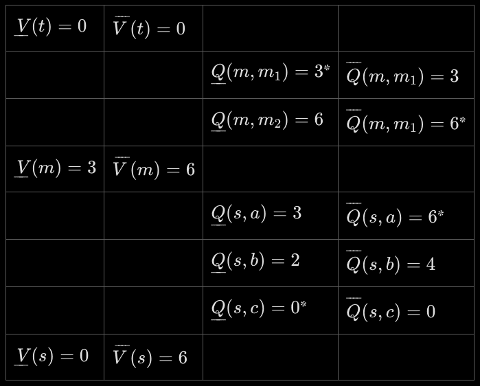
(The asterisks* mark which actions give the $V$ values)

Suppose that the agent is in the initial state $s$ and has the aspiration $E (s) = 2.5$ .

First, we calculate the action-aspirations: if I were to take a certain action, what would I aspire to? Here, the state-aspiration $E (s)$ lies within the action’s feasibility set $Q (s, b)$ , so the action-aspiration $E (s, b)$ is simply set equal to $E (s)$ . By contrast, the intervals $Q (s, a)$ and $Q (s, c)$ do not contain the point $E (s)$ , and so $E (s)$ is clipped to the nearest admissible value:

Fig. 4: Setting action-aspirations in the toy example by clipping state aspiration to actions’ feasibility intervals.

Next, we choose an over-achieving action $a_{+}$ and an under-achieving action $a_{-}$ .
Suppose we arbitrarily choose actions $c$ (do nothing) and $a$ (walk to the market).
We calculate the relative position of the aspiration $E (s)$ between $E (s, c)$ and $E (s, a)$ : $p = E (s, c) ∖ E (s) ∖ E (s, a) = \frac{5}{6}$ .
We roll a die and choose our next action to be either $c$ with probability $1 - p = \frac{1}{6}$ or $a$ with probability $p = \frac{5}{6}$ .
We take the chosen action, walking to the market or doing nothing depending on the result of the die roll, and observe the consequences of our actions! In this case, there are no surprises, as the transitions are deterministic.
We rescale the action-aspiration to determine our new state-aspiration. If we chose action $a$ , we deterministically transitioned to state $m$ , and so the feasibility interval $Q (s, a)$ is equal to $V (m)$ and no rescaling is necessary (in other words, the rescaling is simply the identity map): we simply set our new state-aspiration to be $E (m) = E (s, a) = 3$ . Likewise, if we took action $c$ , we end up in state $t$ with state-aspiration $E (t) = 0$ .

Suppose now that we started with the same initial aspiration $E (s) = 2.5$ , but instead chose action $b$ as our over-achieving action in step 2. In this case, algorithm execution would go as follows:

Determine action-aspirations as before.
Choose $a_{-} = c, a_{+} = b$ .
Since $E (s, b)$ is exactly equal to our state-aspiration $E (s)$ and $E (s, a)$ is not, $p$ is 1!
Hence, our next action is deterministically $b$ .
We execute action $b$ and observe whether public transportation is late today (ending up in state $t$ ) or not (which brings us to state $m$ ).
For the rescaling, we determine the relative position of our action-aspiration in the feasibility interval: $λ = Q - - (s, b) ∖ E (s, b) ∖ ¯ ¯¯ ¯ Q (s, b) = 1 / 4$ .
If we ended up in state $m$ , our new state-aspiration is then $E (m) = V - - (m) : λ : ¯ ¯¯ ¯ V (m) = 3.75$ ; if we ended up in state $t$ , the state-aspiration is $E (t) = 0$ .

These examples demonstrate two cases:

If neither of the action feasibility intervals $Q (a_{+})$ nor $Q (a_{-})$ contain the state aspiration $E (s)$ , we choose between taking action $a_{+}$ and henceforth minimizing, or taking action $a_{-}$ and henceforth maximizing, with the probability $p$ that makes the expected total match our original aspiration $E (s)$ .
If exactly one of the feasibility intervals $Q (s, a_{+})$ or $Q (s, a_{-})$ contains $E (s)$ , then we choose the corresponding action with certainty, and propagate the aspiration by rescaling it.

There is one last case, where both feasibility intervals contain $E (s)$ ; this is the case, for example, if we choose $E (s) = 3.5$ in the above environment. Execution then proceeds as follows:

We determine action-aspirations, as shown here:

Suppose now that we choose actions $a$ and $b$ as $a_{+}$ and $a_{-}$ . (If action $c$ is chosen, then we are in the second case shown above.)
$p$ is defined as the relative position of $E (s)$ between $E (s, a_{-})$ and $E (s, a_{+})$ , but in this case, these three values are equal! We have chosen above (see auxiliary notation) that $p = \frac{1}{2}$ in this case, but any other probability would also be acceptable.
We toss a coin to decide between actions $a$ and $b$ .
The chosen action is performed, either taking us deterministically to the market $m$ if we chose action $a$ or randomizing between $m$ and $t$ if we chose action $b$ .
We propagate the action-aspiration to state-aspiration as before. If we chose action $a$ , then we have $Q (s, a) = V (m)$ and so the new state-aspiration is $E (m) = E (s, a) = 3.5.$ If we chose action $b$ , then the new state-aspiration is $E (m) = V - - (s, m) : \frac{3}{4} : ¯ ¯¯ ¯ V (s, m) = 5.25$ if we reached the market and $E (t) = 0$ otherwise.

Now that we have an idea of how the decision algorithm works, it is time to prove its correctness.

Theorem: Algorithm 1 fulfills the goal

If the world model predicts state transitions correctly and the episode-aspiration $E (s_{0})$ is in the initial state’s feasibility interval, $E (s_{0}) \in V (s_{0})$ , then decision algorithm 1 fulfills the goal $E τ = E (s_{0})$ .

Proof.

First, let us observe that algorithm 1 preserves feasibility: if we start from state $s_{0}$ with state-aspiration $E (s_{0}) \in V (s_{0})$ , then for all states $s$ and actions $a$ visited, we will have $E (s_{0}) \in V (s_{0})$ and $E (s, a) \in Q (s, a)$ .
This statement is easily seen to be true for action-aspirations, as they are required to be feasible by definition in step 1, and correctness for state-aspirations follows from the definition of $E (s^{'})$ in step 6.

Let us now denote by $V^{π_{1}} (s, e)$ the expected Total obtained by algorithm 1 starting from state $s$ with state-aspiration $E (s) = e$ , and likewise by $Q^{π_{1}} (s, a, e)$ the expected Total obtained by starting at step 5 in algorithm 1 with action-aspiration $E (s, a) = e$ .

Since the environment is assumed to be acyclic and finite, we can straightforwardly prove the following claims by backwards induction:

For any state $s$ and any state-aspiration $E (s)$ belonging to the feasibility interval $V (s)$ , we indeed have $V^{π_{1}} (s, E (s)) = E (s)$ .
For any state-action pair $(s, a)$ and any action-aspiration $E (s, a)$ belonging to the feasibility interval $Q (s, a)$ , the expected future Total $Q^{π_{1}} (s, a, E (s, a))$ is in fact equal to $E (s, a)$ .

We start with claim 1. The core reason why this is true is that, for non-terminal states $s$ , we chose the right $p$ in step 3 of the algorithm: $\begin{matrix} V^{π_{1}} (s, E (s)) & = (1 - p) \cdot Q^{π_{1}} (s, a_{-}, E (s, a_{-})) + p \cdot Q^{π_{1}} (s, a_{+}, E (s, a_{+})) = (1 - p) \cdot E (s, a_{-}) + p \cdot E (s, a_{+}) by induction hypothesis = E (s, a_{-}) : p : E (s, a_{+}) = E (s) because p = E (s, a_{-}) ∖ E (s) ∖ E (s, a_{+}) . \end{matrix}$

Claim 1 also serves as the base case for our induction: if $s$ is a terminal state, then $Q (s)$ is an interval made up of a single point, and in this case claim 1 is trivially true.

Claim 2 requires that the translation between action-aspirations, chosen before the world’s reaction is observed, and subsequent state-aspirations, preserves expected Total. The core reason why this works is the linearity of the rescaling operations in step 6:

$\begin{matrix} Q^{π_{1}} (s, a, E (s, a)) = \sum s^{'} \in S P_{M} (s^{'} ∣ s, a) (E δ (s, a, s^{'}) + V^{π_{1}} (s^{'}, E (s^{'}))) assuming correct worldmodel = \sum s^{'} P_{M} (s^{'} ∣ s, a) \cdot (E δ (s, a, s^{'}) + E (s^{'})) by induction hypothesis = \sum s^{'} P_{M} (s^{'} ∣ s, a) \cdot (E δ (s, a, s^{'}) + V - - (s^{'}) : λ : ¯ ¯¯ ¯ V (s^{'})) by definition in step 6 = \sum s^{'} P_{M} (s^{'} ∣ s, a) \cdot ((E δ (s, a, s^{'}) + V - - (s^{'})) : λ : (E δ (s, a, s^{'}) ¯ ¯¯ ¯ V (s^{'}))) = (\sum s^{'} P_{M} (s^{'} ∣ s, a) \cdot (E δ (s, a, s^{'}) + V - - (s^{'}))) : λ : (\sum s^{'} P_{M} (s^{'} ∣ s, a) \cdot (E δ (s, a, s^{'}) ¯ ¯¯ ¯ V (s^{'}))) = Q - - (s, a) : λ : ¯ ¯¯ ¯ Q (s, a) using the Bellman equation for Q = E (s, a) because λ = Q - - (s, a) ∖ E (s, a) ∖ ¯ ¯¯ ¯ Q (s, a) by definition \end{matrix}$

This concludes the correctness proof of algorithm 1. $□$

Notes

It might seem counterintuitive that the received Delta (or at least the expected Delta) is never explicitly used in propagating the aspiration. The proof above however shows that it is implicitly used when rescaling from $Q (s, a)$ (which contains $E_{s^{'}} δ (s, a, s^{'})$ ) to $V (s^{'})$ (which does not contain it any longer).
We clip the state aspiration to the actions’ feasibility intervals to keep the variability of the resulting realized Total low. If the state aspiration is already in the action’s feasibility interval, this does not lead to extreme actions. However, if it is outside an action’s feasibility interval, it will be mapped onto one endpoint of that interval, so if that action is actually chosen, the subsequent behavior will coincide with a maximizer’s or minimizer’s behavior from that point on.
The intervals $V (s)$ and $Q (s, a)$ used for clipping and rescaling can also be defined in various other ways than equation (F) to avoid taking extreme actions even more, e.g., by using two other, more moderate reference policies than the maximizer’s and minimizer’s policy.
Rather than clipping the state aspiration to an action’s feasibility interval, one could also rescale it from the state’s to the action’s feasibility interval, $E^{'} (s, a) \leftarrow Q - - (s, a) : (V - - (s) ∖ E (s) ∖ ¯ ¯¯ ¯ V (s)) : ¯ ¯¯ ¯ Q (s, a)$ . This would avoid extreme actions even more, but would overly increase the variability of received Total even in very simple environments.
Whatever rule the agent uses to set action-aspirations and choose candidate actions, it should be for each action independently, because looking at all possible pairs or even all subsets or lotteries of actions would increase the algorithm’s time complexity more than we think is acceptable if we want it to remain tractable. (We tackle the question of algorithm complexity in the main sequence).

What can we do with this?

We can extend the basic algorithm by adding criteria for choosing the two candidate actions the algorithm mixes, and by generalizing the goal from making the expected Total equal a particular value to making it fall into a particular interval.

The interesting question now is what criteria the agent should use to pick the two candidate actions $a_{-}, a_{+}$ in step 2. We might use this freedom to choose actions in a way that increases safety, e.g., by choosing randomly as a form a “soft optimization” or by incorporating safety criteria like limiting impact.

Let’s look at some simple illustrative examples of performance and safety criteria (More useful criteria will be discussed in the full LW sequence).

Using the gained freedom to increase safety

After having introduced the basic structure of our decision algorithms we will focus on the core question: How shall we make use of the freedom gained from having aspiration-type goals rather than maximization goals?

After all, while there is typically only a single policy that maximize some objective function (or very few, more or less equivalent policies), there is typically a much larger set of policies that fulfill some constraints (such as the aspiration to make the expected Total equal some desired value).

More formally: Let us think of the space of all (probabilistic) policies, $Π$ , as a compact convex subset of a high-dimensional vector space with dimension $d ≫ 1$ and Lebesgue measure $μ$ . Let us call a policy $π \in Π$ successful iff it fulfills the specified goal, $G$ , and let $Π_{G} \subseteq Π$ be the set of successful policies. Then this set has typically zero measure, $μ (Π_{G}) = 0$ , and low dimension, $d i m (Π_{G}) ≪ d$ , if the goal is a maximization goals, but it has large dimension, $d i m (Π_{G}) \approx d$ , for most aspiration-type goals.

E.g., if the goal is to make expected Total equal an aspiration value, $E τ = E$ , we typically have $d i m (Π_{G}) = d - 1$ but still $μ (Π_{G}) = 0$ . At the end of this post, we discuss how the set of successful policies can be further enlarged by switching from aspiration values to aspiration intervals to encode goals, which makes the set have full dimension, $d i m (Π_{G}) = d$ , and positive measure, $μ (Π_{G}) > 0$ .

What does that mean? It means we have a lot of freedom to choose the actual policy $π \in Π_{G}$ that the agent should use to fulfill an aspiration-type goal. We can try to use this freedom to choose policies that promise to be rather safe than unsafe according to some generic safety metric, similar to the impact metrics used in reward function regularization for maximizers.

Depending on the type of goal, we might also want to use this freedom to choose policies that fulfill the goal in a rather desirable than undesirable way according to some goal-related performance metric.

In this post, we will illustrate this with only very few, “toy” safety metrics, and one rather simple goal-related performance metric, to exemplify how such metrics might be used in our framework. In the LW sequence we discuss more sophisticated and hopefully more useful safety metrics.

Let us begin with a simple goal-related performance metric since that is the most straightforward.

Simple example of a goal-related performance metric

Recall that in step 2 of the basic algorithm, we could make the agent pick any action $a_{-}$ whose action-aspiration is at most as large as the current state-aspiration, $E (s, a_{-}) \leq E (s)$ , and it can also pick any other action, $a_{+}$ , whose action-aspiration is at least as large as the current state-aspiration, $E (s, a_{+}) \geq E (s)$ . This flexibility is because in steps 3 and 4 of the algorithm, the agent is still able to randomize between these two actions $a_{-}, a_{+}$ in a way that makes expected Total, $E τ$ , become exactly $E (s)$ .

If one had an optimization mindset, one might immediately get the idea to not only match the desired expectation for the Total, but also to minimize the variability of the Total, as measured by some suitable statistic such as its variance. In a sequential decision making situation like an MDP, estimating the variance of the Total requires a recursive calculation that anticipates future actions, which can be done but is not trivial (see the LW sequence).

Let us instead look at a simpler metric to illustrate the basic approach: the (relative, one-step) squared deviation of aspiration, which is very easy to compute:

S D A (s, a) := \frac{(E (s, a) - E (s))^{2}}{(¯ ¯¯ ¯ V (s) - V - - (s))^{2}} \in [0, 1] .

The rationale for this is that at any time, the action aspirations $E (s, a_{\pm})$ are the expected values of Total-to-go conditional on taking action $a_{\pm}$ , so keeping them close to $E (s)$ will tend to lead to a smaller variance. Indeed, that variance is lower bounded by $(E (s, a_{-}) - E (s))^{2} : p : (E (s, a_{+}) - E (s))^{2}$ , where $p$ is the probability for choosing $a_{+}$ calculated in step 3 of Algorithm 1.

If the action space is rich enough, there will often be at least one action the action-aspiration of which equals the state-aspiration, $E (s, a) = E (s)$ , because the state-aspiration is contained in that action’s feasibility interval, $E (s) \in Q (s, a)$ . There might even be a large number of such actions. This will in particular be the case in the early steps of an episode. This is because often one can distribute the amount of effort spent on a task more or less flexibly over time; as long as there is enough time left, one might start by exerting little effort and then make up for this in later steps, or begin with a lot of effort and then relax later.

If this is the case, then minimizing $S D A (s, a)$ simply means choosing one of the actions for which $E (s) \in Q (s, a)$ and thus $E (s, a) = E (s)$ and thus $S D A (s, a) = 0$ , and then put $a_{-} = a_{+} = a$ . When there are many such candidate actions $a$ , that will still leave us with some remaining freedom for incorporating some other safety criteria to choose between them, maybe deterministically. One might thus think that this form of optimization is safe enough and should be performed because it gets rid of all variability and randomization in that step.

For example: Assume the goal is to get back home with fourteen apples within a week, and the agent can harvest or eat at most six apples on each day (apples are really scarce). Then each day the agent might choose to harvest or eat any number of apples, as long as its current stock of apples does not deviate from fourteen by more than six times the remaining number of days. Only in the last several days it might then have to harvest or eat exactly six apples per day, to make up for earlier deviations and to land at fourteen apples sharp eventually.

But there’s at least two objections to minimizing SDA. First, generically, we can not be sure enough that there will indeed be many different actions for which $E (s) \in Q (s, a)$ , and so restricting our choice to the potentially only few actions that fulfill this might not allow us to incorporate safety criteria to a sufficient level. In particular, we should expect that the latter is often the case in the final steps of an episode, where there might at best be a single such action that perfectly makes up for the earlier under- or over-achievements, or even no such action at all. Second, getting rid of all randomization goes against the intuition of some many members of our project team that randomization is a desirable feature that tends to increase rather than decrease safety (this intuition also underlies the alternative approach of quantilization).

We think that one should thus not minimize performance metrics such as SDA or any other of the later discussed metrics, but at best use them as soft criteria. Arguably the most standard way to do this is to use a softmin (Boltzmann) policy for drawing both candidate actions $a_{-}$ and $a_{+}$ independently of each other, on the basis of their $S D A$ (or another metric’s) scores:

a_{\pm} \sim exp (- β \times S D A (s, a_{\pm}))

restricted to those $a_{-}, a_{+}$ with $Q (s, a_{-}) \leq Q (s) \leq Q (s, a_{+})$ , and for some sufficiently small inverse temperature $β > 0$ to ensure sufficient randomization.

While the SDA criterion is about keeping the variance of the Total rather low and is thus about fulfilling the goal in a presumably more desirable way from the viewpoint of the goal-setting client, the more important type of action selection criterion is not goal- but safety-related. So let us now look at the latter type of criterion.

Toy example of a generic safety metric

As the apple example above shows, the agent might easily get into a situation where it seems to be a good idea to take an extreme action. A very coarse but straightforward and cheap to compute heuristic for detecting at least some forms of extreme actions is when the corresponding aspiration is close to an extreme value of the feasibility interval: $E (s, a) \approx Q - - (s, a)$ or $E (s, a) \approx ¯ ¯¯ ¯ Q (s, a)$ .

This motivates the following generic safety criterion, the (relative, one-step) squared extremity of aspiration:

S E A (s, a) := 4 \times {((Q - - (s, a) ∖ E (s, a) ∖ ¯ ¯¯ ¯ Q (s, a)) - 1 / 2)}^{2} \in [0, 1] .

(The factor 4 is for normalization only)

The rationale is that using actions $a_{-}, a_{+}$ with rather low values of SEA would tend to make the agent’s aspirations stay close to the center of the relevant feasibility intervals, and thus hopefully also make its actions remain moderate in terms of the achieved Total.

Let’s see whether that hope is justified by studying what minimizing SEA would lead to in the above apple example:

On day zero, $E (s_{0}) = 14$ , $V (s) = [- 42, 42]$ , and $Q (s_{0}, a) = [a - 36, a + 36]$ for $a \in {- 6, \dots, 6}$ . Since the current state-aspiration, 14, is in all actions’ feasibility intervals, all action-aspirations are also 14. Both the under- and overachieving action with smallest SEA is thus $a_{-} = a_{+} = 6$ , since this action’s Q-midpoint, 6, is closest to its action-aspiration, 14. The corresponding $λ = - 30 ∖ 14 ∖ 42 = 44 / 72$ .
On the next day, the new feasibility interval is $V (s_{1}) = [- 36, 36]$ , so the new state-aspiration is $E (s_{1}) = - 36 : 44 / 72 : 36 = 8$ . This is simply the difference between the previous state-aspiration, 14, and the received Delta, 6. (It is easy to see that the aspiration propagation mechanism used has this property whenever the environment is deterministic). Since $Q (s_{1}, a) = [a - 30, a + 30] ∋ 8$ , we again have $E (s_{1}, a) = 8$ for all $a$ , and thus again $a_{-} = a_{+} = 6$ since 6 is closest to 8.
On the next day, $E (s_{2}) = 8 - 6 = 2$ , $Q (s_{2}, a) = [a - 24, a + 24] ∋ 2$ , and now $a_{-} = a_{+} = 2$ since 2 is closest to 2. Afterwards, the agent neither harvests not eats any apples but lies in the grass, relaxing.

The example shows that the consequence of minimizing SEA is not, as hoped, always an avoidance of extreme actions. Rather, the agent chooses the maximum action in the first two steps (which might or might not be what we eventually consider safe, but is certainly not what we hoped the criterion would prevent).

Maybe we should compare Deltas rather than aspirations if we want to avoid this? So what about (relative, one-step) squared extremity of Delta,

S E D (s, a) := 4 \times {((min a^{'} E δ (s, a^{'}) ∖ E δ (s, a) ∖ max a^{'} E δ (s, a^{'})) - 1 / 2)}^{2} \in [0, 1],

If the agent minimizes this instead of SEA in the apple example, it will procrastinate by choosing $a_{-} = a_{+} = 0$ for the first several days, as long as $14 \in Q (s_{t}, 0) = [6 t - 36, 36 - 6 t]$ . This happens on the first four days. On the fifth day ( $t = 4$ ), it will still have aspiration 14. It will then again put $a_{-} = 0$ with action-aspiration $E (s_{4}, 0) = 12 = ¯ ¯¯ ¯ Q (s_{4}, 0)$ , but it will put $a_{+} = 2$ with action-aspiration $E (s_{4}, 2) = 14$ . Since the latter equals the state-aspiration, the calculated probability in step 3 of the algorithm turns out to be $p = 1$ , meaning the agent will use action $a_{+}$ for sure after all, rather than randomizing it with $a_{-}$ . This leaves an aspiration of $14 - 2 = 12$ . On the remaining two days, the agent then has to use $a = 6$ to fulfill the aspiration in expectation.

Huh? Even though both heuristics seem to be based on a similar idea, one of them leads to early extreme action and later relaxation, and the other to procrastination and later extreme action, just the opposite. Neither of them avoids extreme actions.

One might think that one could fix the problem by simply adding the two metrics up into a combined safety loss,

L (s, a) := S E A (s, a) + S E D (s, a) \in [0, 2] .

But in the apple example, the agent would still harvest six apples on the first day, since $(14 - 6)^{2} + (6 - 0)^{2} < (14 - 5)^{2} + (5 - 0)^{2}$ . Only on the second day, it would harvest just four instead of six apples, because $(8 - 4)^{2} + (4 - 0)^{2}$ is minimal. On the third day: two apples because $(4 - 2)^{2} - (2 - 0)^{2}$ is minimal. Then one apple, and then randomize between one or zero apples, until it has the 14 apples, or until the last day has come where it needs to harvest one last apple.

The main reason for all these heuristics failing in that example is their one-step nature which does not anticipate later actions. In the LW sequence we will talk about more complex, farsighted metrics that can still be computed efficiently in a recursive manner, such as disordering potential,

\begin{matrix} D P (s, a) & = E_{s^{'} | s, a} (- log P (s^{'} | s, a) + log \sum a exp (D P (s, a))), \end{matrix}

which measures the largest Shannon entropy in the state trajectory that the agent could cause if it aimed to, or terminal state distance,

\begin{matrix} T S D (s, a, E (s, a)) & = E s^{'} | s, a (1_{s^{'} is terminal} d (s^{'}, s_{0}) + 1_{s^{'} is not terminal} E a^{'} \sim π (s^{'}, E (s^{'})) T S D (s^{'}, a^{'}, E (s^{'}, a^{'}))), \end{matrix}

which measures the expected distance between the terminal and initial state according to some metric $d$ on state space and depends on the actual policy $π$ and aspiration propagation scheme $E (s) \to E (s, a) \to E (s^{'})$ that the agent uses.

Let us finish this post by discussing other ways to combine several performance and/or safety metrics.

Using several safety and performance metrics

Defining a combined loss function like $L (s, a)$ above by adding up components is clearly not the only way to combine several safety and/or performance metrics, and is maybe not the best way to do that because it allows unlimited trade-offs between the components.

It also requires them to be measured in the same units and to be of similar scale, or to make them so by multiplying them with suitable prefactors that would have to be justified. This at least can always be achieved by some form of normalization, like we did above to make SEA and SED dimensionless and bounded by $[0, 1]$ .

Trade-offs between several normalized loss components $L_{i} (s, a) \in [0, 1]$ can be limited in all kinds of ways, for example by using some form of economics-inspired “safety production function” such as the CES-type function

L (s, a) = 1 - {(\sum i b_{i} (1 - L_{i} (s, a))^{ρ})}_{i}^{1 / ρ}

with suitable parameters $ρ$ and $b_{i} > 0$ with $\sum_{i} b_{i} = 1$ . For $ρ = 1$ , we just have a linear combination that allows for unlimited trade-offs. At the other extreme, in the limit of $ρ \to - \infty$ , we get $L (s, a) = {max}_{i} L_{i} (s, a)$ , which does not allow for any trade-offs.

Such a combined loss function can then be used to determine the two actions $a_{-}, a_{+}$ , e.g., using a softmin policy as suggested above.

An alternative to this approach is to use some kind of filtering approach to prevent unwanted trade-offs. E.g., one could use one of the safety loss metrics, $L_{1} (s, a)$ , to restrict the set of candidate actions to those with sufficiently small loss, say with $L_{1} (s, a) \leq {min}_{a^{'}} L_{1} (s, a^{'}) : 0.1 : {max}_{a^{'}} L_{1} (s, a^{'})$ , then use a second metric, $L_{2}$ , to filter further, and so on, and finally use the last metric, $L_{k}$ , in a softmin policy.

One can come up with many plausible generic safety criteria (see LW sequence), and one might be tempted to just combine them all in one of these ways, in the hope to thereby have found the ultimate safety loss function or filtering scheme. But it might also well be that one will have forgotten some safety aspects and end up with an imperfect combined safety metric. This would be just another example of a misspecified objective function. Hence we should again resist falling into the optimization trap of strictly minimizing that combined loss function, or the final loss function of the filtering scheme. Rather, the agent should probably still use a sufficient amount of randomization in the end, for example by using a softmin policy with sufficient temperature.

If it is unclear what a sufficient temperature is, one can set the temperature automatically so that the odds ratio between the least and most likely actions equals a specified value: $β := η / ({max}_{a} L (s, a) - {min}_{a} L (s, a))$ for some fixed $η > 0$ .

More freedom via aspiration intervals

We saw earlier that if the goal is to make expected Total equal an aspiration value, $E τ = E \in R$ , the set of successful policies has large but not full dimension and thus still has measure zero. In other words, making expected Total exactly equal to some value still requires policies that are very “precise” and in this regard very “special” and potentially dangerous. So we should probably allow some leeway, which should not make any difference in almost all real-world tasks but increase safety further by avoiding solutions that are too special.

Of course the simplest way to provide this leeway would be to just get rid of the hard constraint altogether and replace it by a soft incentive to make $E τ$ close to $E \in R$ , for example by using a softmin policy based on the mean squared error. This might be acceptable for some tasks but less so for others. The situation appears to be somewhat similar to the question of choosing estimators in statistics (e.g., a suitable estimator of variance), where sometimes one only wants the estimator with the smallest standard error, not caring for bias (and thus not having any guarantee about the expected value), sometimes one wants an unbiased estimator (i.e., an estimator that comes with an exact guarantee about the expected value), and sometimes one wants at least a consistent estimator that is unbiased in the limit of large data and only approximately unbiased otherwise (i.e., have only an asymptotic rather than an exact guarantee about the expected value).

For tasks where one wants at least some guarantee about the expected Total, one can replace the aspiration value by an aspiration interval $E = [e -, ¯ ¯ ¯ e] \subseteq R$ and require that $E τ \in E$ .

The basic algorithm (algorithm 1) can easily be generalized to this case and only becomes a little bit more complicated due to the involved interval arithmetic:

Decision algorithm 2

Similar to algorithm 1, we…

set action-aspiration intervals $E (s, a) = [e - (s, a), ¯ ¯ ¯ e (s, a)] \subseteq Q (s, a)$ for each possible action $a \in A$ on the basis of the current state-aspiration interval $E (s) = [e - (s), ¯ ¯ ¯ e (s)]$ and the action’s feasibility interval $Q (s, a)$ , trying to keep $E (s, a)$ similar to and no wider than $E (s)$ ,
choose an “under-achieving” action $a_{-}$ and an “over-achieving” action $a_{+}$ w.r.t. the midpoints of the intervals $E (s)$ and $E (s, a)$ ,
choose probabilistically between $a_{-}$ and $a_{+}$ with suitable probabilities, and
propagate the action-aspiration interval $E (s, a)$ to the new state-aspiration interval $E (s^{'})$ by rescaling between the feasibility intervals of $a$ and $s^{'}$ .

More precisely: Let $m (I)$ denote the midpoint of interval $I$ . Given state $s$ and state-aspiration interval $E (s)$ ,

For all $a \in A$ , let $E (s, a)$ be the closest interval to $E (s)$ that lies within $Q (s, a)$ and is as wide as the smaller of $E (s)$ and $Q (s, a)$ .
Pick some $a_{-}, a_{+} \in A$ with $m (E (s, a_{-})) \leq m (E (s)) \leq m (E (s, a_{+}))$
Compute $p \leftarrow m (E (s, a_{-})) ∖ m (E (s)) ∖ m (E (s, a_{-}))$
With probability $p$ , put $a \leftarrow a_{+}$ , otherwise put $a \leftarrow a_{-}$
Implement action $a$ in the environment and observe successor state $s^{'} \leftarrow s t e p (s, a)$
Compute $λ - - \leftarrow Q - - (s, a) ∖ e - (s, a) ∖ ¯ ¯¯ ¯ Q (s, a)$ and $e - (s^{'}) \leftarrow V - - (s^{'}) : λ - - : ¯ ¯¯ ¯ V (s^{'})$ , and similarly for $¯ ¯ ¯ λ$ and $¯ ¯ ¯ e (s^{'})$

Note that the condition that no $E (s, a)$ must be wider than $E (s)$ in step 1 ensures that, independently of what the value of $p$ computed in step 3 will turn out to be, any convex combination $q_{-} : p : q_{+}$ of values $q_{\pm} \in E (s, a_{\pm})$ is an element of $E (s)$ . This is the crucial feature that ensures that aspirations will be met:

Theorem (Interval guarantee)

If the world model predicts state transition probabilities correctly and the episode-aspiration interval $E (s_{0})$ is a subset of the initial state’s feasibility interval, $E (s_{0}) \subseteq V (s_{0})$ , then algorithm 2 fulfills the goal $E τ \in E (s_{0})$ .

The Proof is completely analogous to the last one, except that each occurrence of $V (s, e) = E (s) \in V (s)$ and $Q (s, a, e) = E (s, a) \in Q (s, a)$ is replaced by $V (s, e) \in E (s) \subseteq V (s)$ and $Q (s, a, e) \in E (s, a) \subseteq Q (s, a)$ , linear combination of sets is defined as $c X + c^{'} X^{'} = {c x + c^{'} x^{'} : x \in X, x^{'} \in X^{'}}$ , and we use the fact that $m (E (s, a_{-})) : p : m (E (s, a_{+})) = m (E (s))$ implies $E (s, a_{-}) : p : E (s, a_{+}) \subseteq E (s)$ .

Special cases

Satisficing. The special case where the upper end of the aspiration interval coincides with the upper end of the feasibility interval leads to a form of satisficing guided by additional criteria.

Probability of ending in a desirable state. A subcase of satisficing is when all Deltas are 0 except for some terminal states where it is 1, indicating that a “desirable” terminal state has been reached. In that case, the lower bound of the aspiration interval is simply the minimum acceptable probability of ending in a desirable state.

Glossary

This is how we use certain potentially ambiguous terms in this post:

Agent: We employ a very broad definition of “agent” here: The agent is a machine with perceptors that produce observations, and actuators that it can use to take actions, and that uses a decision algorithm to pick actions that it then takes. Think: a household’s robot assistant, a firm’s or government’s strategic AI consultant. We do not assume that the agent has a goal of its own, let alone that it is a maximizer.

Aspiration: A goal formalized via a set of constraints on the state or trajectory or probability distribution of trajectories of the world. E.g., “The expected position of the spaceship in 1 week from now should be the L1 Lagrange point, its total standard deviation should be at most 100 km, and its velocity relative to the L1 point should be at most 1 km/h”.

Decision algorithm: A (potentially stochastic) algorithm whose input is a sequence of observations (that the agent’s perceptors have made) and whose output is an action (which the agent’s actuators then take). A decision algorithm might use a fixed “policy” or a policy it adapts from time to time, e.g. via some form of learning, or some other way of deriving a decision.

Maximizer: An agent whose decision algorithm takes an objective function and uses an optimization algorithm to find the (typically unique) action at which the predicted expected value of the objective function (or some other summary statistic of the predicted probability distribution of the values of this function) is (at least approximately) maximal, and then outputs that action.

Optimization algorithm: An algorithm that takes some function $f$ (given as a formula or as another algorithm that can be used to compute values $f (x)$ of that function), calculates or approximates the (typically unique) location $x$ of the global maximum (or minimum) of $f$ , and returns that location $x$ . In other words: an algorithm $O : f \mapsto O (f) \approx arg {max}_{x} f (x)$ .

Utility function: A function (only defined up to positive affine transformations) of the (predicted) state of the world or trajectory of states of the world that represents the preferences of the holder of the utility function over all possible probability distributions of states or trajectories of the world in a way conforming to the axioms of expected utility theory or some form of non-expected utility theory such as cumulative prospect theory.

Loss function: A non-negative function of potential outputs of an algorithm (actions, action sequences, policies, parameter values, changes in parameters, etc.) that is meant to represent something the algorithm shall rather keep small.

Goal: Any type of additional input (additional to the observations) to the decision algorithm that guides the direction of the decision algorithm, such as:

a desirable state of the world or trajectory of states of the world, or probability distribution over trajectories of states of the world, or expected value for some observable
a (crisp or fuzzy) set of acceptable states, trajectories, distributions of such, or expected value of some observable
a utility function for expected (or otherwise aggregated) utility maximization

Planning: The activity of considering several action sequences or policies (“plans”) for a significant planning time horizon, predicting their consequences using some world model, evaluating those consequences, and deciding on one plan the basis of these evaluations.

Learning: Improving one’s beliefs/knowledge over time on the basis of some stream of incoming data, using some form of learning algorithm, and potentially using some data acquisition strategy such as some form of exploration.

Satisficing: A decision-making strategy that entails selecting an option that meets a predefined level of acceptability or adequacy rather than optimizing for the best possible outcome. This approach emphasizes practicality and efficiency by prioritizing satisfactory solutions over the potentially exhaustive search for the optimal one. See also the satisficer tag.

Quantilization: A technique in decision theory, introduced in a 2015 paper by Jessica Taylor. Instead of selecting the action that maximizes expected utility, a quantilizing agent chooses randomly among the actions which rank higher than a predetermined quantile in some base distribution of actions. This method aims to balance between exploiting known strategies and exploring potentially better but riskier ones, thereby mitigating the impact of errors in the utility estimation. See also the quantilization tag.

Reward Function Regularization: A method in machine learning and AI design where the reward function is modified by adding penalty terms or constraints to discourage certain behaviors or encourage others, such as in Impact Regularization. This approach is often used to incorporate safety, ethical, or other secondary objectives into the optimization process. As such, it can make use of the same type of safety criteria as an aspiration-based algorithm might.

Safety Criterion: A (typically quantitative) formal criterion that assesses some potentially relevant safety aspect of a potential action or plan. E.g., how much change in the world trajectory could this plan maximally cause? Safety criteria can be used as the basis of loss functions or in reward function regularization to guide behavior.

Using Aspirations as a Means to Maximize Reward: An approach in adaptive reinforcement learning where aspiration levels (desired outcomes or benchmarks) are adjusted over time based on performance feedback. Here, aspirations serve as dynamic targets to guide learning and action selection towards ultimately maximizing cumulative rewards. This method contrasts with using aspirations as fixed goals, emphasizing their role as flexible benchmarks in the pursuit of long-term utility optimization. This is not what we assume in this project, where we assume no such underlying utility function.

Project status

The SatisfIA project is a collaborative effort by volunteers from different programs: AI Safety Camp, SPAR, and interns from different ENSs, led by Jobst Heitzig at PIK’s Complexity Science Dept. and the FutureLab on Game Theory and Networks of Interacting Agents that has started to work on AI safety in 2023.

Motivated by the above thoughts, two of us (Jobst and Clément) began to investigate the possibility of avoiding the notion of utility function altogether and develop decision algorithms based on goals specified through constraints called “aspirations”, to avoid risks from Goodhart’s law and extreme actions. We originally worked in a reinforcement learning framework, modifying existing temporal difference learning algorithms, but soon ran into issues more related to the learning algorithms than to the aspiration-based policies we actually wanted to study (see Clément’s earlier post).

Because of these issues, discussions at VAISU 2023 and FAR Labs, and comments from Stuart Russell, Jobst then switched from a learning framework to a model-based planning framework and adapted the optimal planning algorithms from agentmodels.org to work with aspirations instead, which worked much better and allowed us to focus on the decision making aspect.

As of spring 2024, the project is participating in AI Safety Camp and SPAR with about a dozen people investing a few hours a week. We are looking for additional collaborators. Currently, our efforts focus on theoretical design, prototypical software implementation, and simulations in simple test environments. We will continue documenting our progress in the LW sequence. We also plan to submit a first academic conference paper soon.

Acknowledgements

In addition to AISC, SPAR, VAISU, FAR Labs, and GaNe, we’d like to thank everyone who contributed or continues to contribute to the SatisfIA project.

^
The algorithm is based on the idea of propagating aspirations along time, and we prove that the algorithm gives a performance guarantee if the goal is feasible. Then we extend the basic algorithm by 1) adding criteria for choosing the two candidate actions the algorithm mixes, and 2) by generalizing the goal from making the expected Total equal a particular value to making it fall into a particular interval.
^
This might not be trivial of course if the agent might “outsource” or otherwise cause the maximization of some objective function by others, a question that is related to “reflective stability” in the sense of this post. An rule additional “do not maximize” would hence be something like “do not cause maximization by other agents”, but this is beyond the scope of the project at the moment.
^
Information-theoretic, not thermodynamic.
^
This is also why Sutton and Barto’s leading textbook on RL starts with model-based algorithms and turns to learning only in chapter 6.
^
When we extend our approach later to incorporate performance and safety criteria, we might also have to assume further functions, such as the expected squared Delta (to be able to estimate the variance of Total), or some transition-internal world trajectory entropy (to be able to estimate total world trajectory entropy), etc.
^
Note that this type of goal is also implicitly assumed in the alternative Decision Transformer approach, where a transformer network is asked to predict an action leading to a prompted expected Total.
^
If the agent is a part of a more complex system of collaborating agents (e.g., a hierarchy of subsystems), the “action” might consist in specifying a subtask for another agent, that other agent would be modeled as part of the “environment” here, and the observation returned by $s t e p$ might be what that other agent reports back at the end of its performing that subtask.
^
It is important to note that $s_{t}$ might be an incomplete description of the true environment state, which we denote $x_{t}$ but rarely refer to here.
^
Note that we’re in a model-based planning context, so it directly computes the values recursively using the world model, rather than trying to learn it from acting in the real or simulated environment using some form of reinforcement learning.
^
These assumptions may of course be generalized, at the cost of some hassle in verifying that expectations are well-defined, to allow cycles or infinite time horizons, but the general idea of the proof remains the same.
^
E.g., assume the agent can buy zero or one apple per day, has two days time, and the aspiration is one apple. On the first day, the state’s feasibility interval is $[0, 2]$ , the action of buying zero apples has feasibility interval $[0, 1]$ and would thus get action-aspiration 0.5, and the action of buying one apple has feasibility interval $[1, 2]$ and would thus get action-aspiration 1.5. To get 1 on average, the agent would thus toss a coin. So far, this is fine, but on the next day the aspiration would not be 0 or 1 in order to land at 1 apple exactly, but would be 0.5. So on the second day, the agent would again toss a coin. Altogether, it would get 0 or 1 or 2 apples, with probabilities ¹⁄₄, ¹⁄₂, and ¹⁄₄, rather than getting 1 apple for sure.
^
That the algorithm uses an optimization algorithm that it gives the function to maximize to is crucial in this definition. Without this condition, every agent would be a maximizer, since for whatever output $a$ the decision algorithm produces, one can always find ex post some function $f$ for which $arg {max}_{x} f (x) = a$ .

Aspiration-based, non-maximizing AI agent designs