Famine deaths due to the climatic effects of nuclear war
The views expressed here are my own, not those of Alliance to Feed the Earth in Disasters (ALLFED), for which I work as a contractor. Please assume this is always the case unless stated otherwise.
Summary
The initial motivation for my analysis was combining the results of 2 views about nuclear winter:
One linked to Alan Robock (Rutgers University), Michael Mills (National Center for Atmospheric Research), and Brian Toon (University of Colorado), which is illustrated in Xia 2022. “We estimate more than 2 billion people could die from nuclear war between India and Pakistan, and more than 5 billion could die from a war between the United States and Russia”.
Another linked to Jon Reisner (Los Alamos National Laboratory), which is illustrated in Reisner 2018. “Our analysis demonstrates that the probability of significant global cooling from a limited exchange scenario as envisioned in previous studies is highly unlikely, a conclusion supported by examination of natural analogs, such as large forest fires and volcanic eruptions”.
I estimate 12.9 M expected famine deaths due to the climatic effects of nuclear war before 2050, multiplying:
3.30 % probability of large nuclear war before 2050, multiplying:
392 M famine deaths due to the climatic effects of a large nuclear war, multiplying:
4.43 % famine death rate due to the climatic effects for 22.1 Tg (22.1 trillion grams, i.e. million tonnes[1]) of soot injected into the stratosphere in a large nuclear war, multiplying:
2.09 k offensive nuclear detonations in a large nuclear war.
21.5 % countervalue nuclear detonations.
0.0491 Tg per countervalue nuclear detonation, multiplying:
189 kt of yield per countervalue nuclear detonation.
2.60*10^-4 Tg/kt of soot injected into the stratosphere per countervalue yield.
My expected annual famine deaths due to the climatic effects of nuclear war before 2050 are 496 k, and my 5th and 95th percentile are 0 and 30.9 M. My 95th percentile is 62.3 times my best guess, which means there is lots of uncertainty. Bear in mind my estimates only refer to the famine deaths due to the climatic effects. I exclude famine deaths resulting directly or indirectly from infrastructure destruction, and heat mortality.
I obtained my best guess for the soot injected into the stratosphere per countervalue yield giving the same weight to results I inferred from Reisner’s and Toon’s views, but they differ substantially. If I attributed all weight to the result I deduced from Reisner’s (Toon’s) view, my estimates for the expected mortality would become 0.121 (8.27) times as large. In other words, my best guess is hundreds of millions of famine deaths due to the climatic effects, but tens of millions putting all weight in the result I deduced from Reisner’s view, and billions putting all weight in the one I deduced from Toon’s view. Further research would be helpful to figure out which view should be weighted more heavily.
My expected famine deaths due to the climatic effects of a large nuclear war are 17.7 M/Tg (per soot injected into the stratosphere) and 0.992 M/Mt (per total yield). These are 32.3 % and 7.81 % of the 54.8 M/Tg and 12.7 M/Mt of Xia 2022, which I deem too pessimistic.
My estimate of 12.9 M expected famine deaths due to the climatic effects of nuclear war before 2050 is 2.05 % the 630 M implied by Luisa Rodriguez’s results for nuclear exchanges between the United States and Russia, so I would say they are significantly pessimistic[3]. I am also surprised by Luisa’s distribution for the famine death rate due to the climatic effects given at least one offensive nuclear detonation in the United States or Russia. Her 5th and 95th percentile are 41.0 % and 99.6 %, which I think are too close and high.
I believe Mike underweighted Reisner’s view.
I guess the famine deaths due to the climatic effects of a large nuclear war would be 1.16 times the direct deaths. Putting all the weight in the soot injected into the stratosphere per countervalue yield I inferred from Reisner’s (Toon’s) view, the famine deaths due to the climatic effects would be 0.140 (9.59) times the direct deaths. In other words, my best guess is that famine deaths due to the climatic effects are within the same order of magnitude of the direct deaths, but 1 order of magnitude lower putting all weight in the result I inferred from Reisner’s view, and 1 higher putting all weight in the one I inferred from Toon’s view.
Combining my mortality estimates with data from Denkenberger 2016, I estimate the expected cost-effectiveness of planning, research and development of resilient food solutions is 28.7 $/life, which is 2 orders of magnitude more cost-effective than GiveWell’s top charities. Nevertheless, I suspect the values from Denkenberger 2016 are very optimistic, such that I am greatly overestimating the cost-effectiveness. I guess the true cost-effectiveness is within the same order of magnitude of that of GiveWell’s top charities, although this adjustment is not resilient. Furthermore, I have argued corporate campaigns for chicken welfare are 3 orders of magnitude more cost-effective than GiveWell’s top charities.
I do not think activities related to resilient food solutions are cost-effective at increasing the longterm value of the future. By not cost-effective, I mostly mean I do not see those activities being competitive with the best opportunities to decrease AI risk, and improve biosecurity and pandemic preparedness at the margin, like Long-Term Future Fund’s marginal grants.
It is often hard to find interventions which are robustly beneficial. In my mind, decreasing the famine deaths due to the climatic effects of nuclear war is no exception, and I think it is unclear whether that is beneficial or harmful from both a nearterm and longterm perspective (although I strongly oppose killing people, including via nuclear war).
Feel free to check my personal recommendations for funders.
Introduction
I have been assuming the importance of the climatic effects of nuclear war is roughly in agreement with Denkenberger 2018 and Luisa’s post, but I had not looked much into the relevant literature myself. I got interested in doing so following some of the discussion in my global warming post, and Bean’s and Mike’s analyses.
The initial motivation for my analysis was combining the results of 2 views about nuclear winter:
One linked to Alan Robock (Rutgers University), Michael Mills (National Center for Atmospheric Research), and Brian Toon (University of Colorado), which is illustrated in Xia 2022. “We estimate more than 2 billion people could die from nuclear war between India and Pakistan, and more than 5 billion could die from a war between the United States and Russia”.
Another linked to Jon Reisner (Los Alamos National Laboratory), which is illustrated in Reisner 2018. “Our analysis demonstrates that the probability of significant global cooling from a limited exchange scenario as envisioned in previous studies is highly unlikely, a conclusion supported by examination of natural analogs, such as large forest fires and volcanic eruptions”.
Denkenberger 2018 did not integrate the results of Reisner 2018, which was published afterwards[4]. Luisa says:
As a final point, I’d like to emphasize that the nuclear winter is quite controversial (for example, see: Singer, 1985; Seitz, 2011; Robock, 2011; Coupe et al., 2019; Reisner et al., 2019; Pausata et al., 2016; Reisner et al., 2018; Also see the summary of the nuclear winter controversy in Wikipedia’s article on nuclear winter). Critics argue that the parameters fed into the climate models (like, how much smoke would be generated by a given exchange) as well as the assumptions in the climate models themselves (for example, the way clouds would behave) are suspect, and may have been biased by the researchers’ political motivations (for example, see: Singer, 1985; Seitz, 2011; Reisner et al., 2019; Pausata et al., 2016; Reisner et al., 2018). I take these criticisms very seriously — and believe we should probably be skeptical of this body of research as a result. For the purposes of this estimation, I assume that the nuclear winter research comes to the right conclusion. However, if we discounted the expected harm caused by US-Russia nuclear war for the fact that the nuclear winter hypothesis is somewhat suspect, the expected harm could shrink substantially.
I also felt like Bean’s analysis underweighted Rutgers’ view, and Michael Hinge’s underweighted Los Alamos’ (see my comments).
My goal is estimating the famine deaths due to the climatic effects of nuclear war, not all famine deaths, nor heat mortality (related to hot or cold exposure). I also:
Do a very shallow analysis of the cost-effectiveness of activities related to resilient food solutions.
Discuss potential negative effects of decreasing famine deaths.
Famine deaths due to the climatic effects
Overview
I arrived at 12.9 M (= 0.0330*392*10^6) famine deaths due to the climatic effects of nuclear war before 2050, multiplying:
3.30 % probability of a large nuclear war before 2050.
392 M famine deaths due to the climatic effects of a large nuclear war, which I determined by multiplying:
Famine death rate due to the climatic effects of a large nuclear war, which I obtained from the soot injected into the stratosphere in a large nuclear war[5]. I calculated this from the product between:
Offensive nuclear detonations in a large nuclear war.
Countervalue nuclear detonations as a fraction of the total.
Soot injected into the stratosphere per countervalue nuclear detonation.
Global population.
Unlike Denkenberger 2018 and Luisa, I did not run a Monte Carlo simulation modelling all non-probabilistic variables as distributions, but I do not think that would meaningfully move my estimate of the expected deaths:
Assuming all 4 factors describing the soot injected into the stratosphere before 2050 given at least one offensive nuclear detonation before 2050 are independent, as I would do for simplicity anyway in a Monte Carlo simulation, the product between their expected values would be the expected product (E(X Y) = E(X) E(Y) if X and Y are independent).
From Fig. 5b of Xia 2022, the number of people without food in year 2 is roughly proportional to the soot injected into the stratosphere[6].
To be precise, from the data on Table 1, the linear regression with null intercept of the former on the latter has a coefficient of determination (R^2) of 96.8 %.
Therefore, since the mean is a linear operator (E(a X + b) = a E(X) + b), one can obtain the expected number of people without food in year 2 from the expected soot injected into the stratosphere.
Christian Ruhl argues for the non-linearity of nuclear war effects. I agree, as I guess starvation deaths increase logistically with the soot injected into the stratosphere, but I believe injections of soot into the stratosphere for large nuclear wars fall in its roughly linear part.
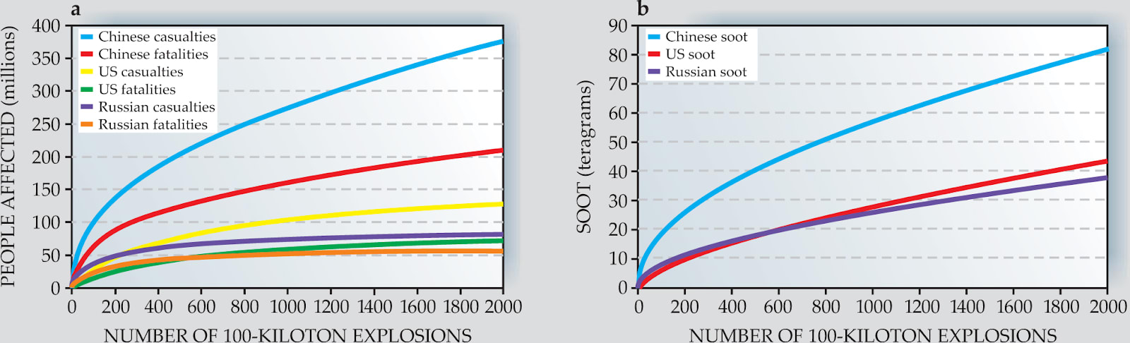
I defined such wars as having at least 1.07 k offensive nuclear detonations, and Figure 2b of Toon 2008, presented below, suggests emitted soot increases linearly with the number of detonations in that case.
If the linear part of the logistic curve starts sooner/later, the starvation resulting from small nuclear wars will tend to be larger/smaller, and therefore I would be underestimating/overestimating expected mortality.
My point estimates respect the expected values, not medians, of the variables to which the result of interest is proportional to.
Probability of large nuclear war
I put the probability of large nuclear war before 2050 at 3.30 % (= 0.32*0.103), which is the product between:
32 % probability of at least one offensive nuclear detonation before 2050.
10.3 % probability of large nuclear war conditional on the above.
I motivate these values below.
Probability of at least one offensive nuclear detonation
I placed the probability of at least one offensive nuclear detonation before 2050 at 32 %, in agreement with Metaculus’ community prediction on 31 August 2023[7]. This is reasonable based on:
The base rate:
There have been offensive nuclear detonations in 1 year (1945) over the 79 (= 2023 − 1945 + 1) during which they could occur. This suggests an annual probability of at least one offensive nuclear detonation of 1.27 % (= 1⁄79).
There are still 26 years (= 2050 − 2024) before 2050.
So the base rate implies a probability of at least one offensive nuclear detonation before 2050 of 28.3 % (= 1 - (1 − 0.0127)^26), which is 88.4 % (= 28.3/32) of Metaculus’ community prediction.
Luisa’s prediction[8]:
1.1 %/year (see table).
25.0 % (= 1 - (1 − 0.011)^26) before 2050, which is 78.1 % (= 25.0/32) of Metaculus’ community prediction.
Probability of escalation into large nuclear war
I presupposed a beta distribution for the fraction of nuclear warheads being detonated before 2050 given at least one offensive nuclear detonation before then. I defined it from 61th and 89th percentiles equal to 1.06 % (= 100/(9.43*10^3)) and 10.6 % (= 1*10^3/(9.43*10^3)), given:
Metaculus’ community predictions on 26 September 2023 of 39 % (= 1 − 0.61) and 11 % (= 1 − 0.89) for the probability of at least 100 and 1 k offensive nuclear detonations before 2050 given at least one offensive nuclear detonation before then.
9.43 k (= (9.50 + (9.22 − 9.50)/(2052 − 2032)*(2037 − 2032))*10^3 − 1) expected nuclear warheads minus 1[9], which I obtained:
For 2037 (= (2050 − 2024)/2), which is midway between now and 2050[10].
Linearly interpolating between the mean of Metaculus’ 25th and 75th percentile community predictions on 11 September 2023 for[11]:
2032, 9.50 k (= (8.29 + 10.7)*10^3/2).
2052, 9.22 k (= (4.84 + 13.6)*10^3/2).
The alpha and beta parameters of the beta distribution are 0.189 and 5.03, and its cumulative distribution function (CDF) is below. The horizontal axis is the fraction of nuclear warheads being detonated, and the vertical one the probability of less than a certain fraction being detonated. The probability of escalation into a large nuclear war, which I defined as at least 1.07 k offensive nuclear detonations, corresponding to 11.3 % (= 1.07*10^3/(9.43*10^3)) of nuclear warheads being detonated, is 10.3 %[12].
Soot injected into the stratosphere
I expect 22.1 Tg (= 2.09*10^3*0.215*0.0491) of soot being injected into the stratosphere in a large nuclear war. This is the product between:
2.09 k offensive nuclear detonations in a large nuclear war.
21.5 % countervalue nuclear detonations[13].
0.0491 Tg (= 189*2.60*10^-4) per countervalue nuclear detonation, multiplying:
189 kt yield per countervalue nuclear detonation.
2.60*10^-4 Tg/kt of soot injected into the stratosphere per countervalue yield.
I explain the above estimates in the next sections. I neglected counterforce nuclear detonations because:
From Figure 4 of Wagman 2020, the soot injected into the stratosphere for an available fuel per area of 5 g/cm^2 is negligible[14].
I estimated an available fuel per area of g/cm^2 for counterforce nuclear detonations of 3.07 g/cm^2, which is lower than the above 5 g/cm^2.
Offensive nuclear detonations
I expect 2.09 k (= 1 + 0.221*9.43*10^3) offensive nuclear detonations in a large nuclear war. This is 1 plus the product between:
22.1 % of nuclear warheads being offensively detonated in a large nuclear war, which I computed:
Generating 1 M Monte Carlo samples of the beta distribution describing the fraction of nuclear warheads being detonated before 2050 given at least one offensive nuclear detonation before then.
Taking the mean of the above samples larger or equal to 11.3 %, which is the minimum fraction for a large nuclear war.
9.43 k expected nuclear warheads minus 1.
The 5th and 95th percentile fraction of nuclear warheads being detonated in a large nuclear war are 11.8 % and 43.6 %, which correspond to 1.11 k (= 1 + 0.118*9.43*10^3) and 4.11 k (= 1 + 0.436*9.43*10^3) offensive nuclear detonations.
I compared the offensive nuclear detonations, given at least one before 2050, implied by my beta distribution with those of a Metaculus’ question whose predictions I ended up not using. The 5th, 50th and 95th percentile of the beta distribution are 1.84*10^-6 %, 0.362 % and 19.2 %[15], and the respective detonations given at least one are:
1.00 (= 1 + 1.84*10^-8*9.43*10^3), which is 90.1 % (= 1.00/1.11) Metaculus’ 5th percentile community prediction of 1.11.
35.1 (= 1 + 0.00362*9.43*10^3), which is 3.97 (= 35.1/8.84) times Metaculus’ median community prediction of 8.84[16] (= (8.56 + 9.11)/2).
1.81 k (= 1 + 0.192*9.43*10^3), which is 21.5 % (= 1.81/8.42) Metaculus’ 95th percentile community prediction of 8.42 k[17] (= (7.18 + 9.66)/2*10^3).
The mean of my beta distribution is 3.62 % (= 0.189/(0.189 + 5.03)), and therefore I expect 342 (= 1 + 0.0362*9.43*10^3) offensive nuclear detonations given one offensive nuclear detonation before 2050, which is 9.74 (= 342⁄35.1) times my median detonations. Additionally, my 95th percentile is 1.81 k (= 1.81*10^3/1.00) times my 5th percentile. Such high ratios illustrate nuclear war is predicted to be heavy-tailed, as has been the case for non-nuclear wars.
From the above bullets, the predictions for the number of detonations I arrived at fitting a beta distribution to the forecasts for 2 Metaculus’ questions about the probability of escalation to large nuclear wars (100 and 1 k detonations) are not quite in line with the forecasts for another Metaculus’ question explicitly about the number of detonations. The large difference for the 95th percentile is relevant because the right tail has a significant influence on the expected detonations, as can be seen from the high ratio between my mean and median detonations. I decided to rely on the 2 Metaculus’ questions about escalation because:
Of the importance of the right tail. The other requires forecasters to estimate the entire probability distribution, which I expect to lead to less accurate forecasts for the right tail.
I would have to arbitrarily select 2 quantiles from the other in order to define the beta distribution.
Countervalue nuclear detonations
I assumed 21.5 % of the offensive nuclear detonations to respect countervalue targeting. This was Metaculus’ median community prediction on 30 September 2023 for the fraction of offensive nuclear detonations before 2050 which will be countervalue.
I presumed 100 % total burned area as a fraction of the burned area assuming different detonations did not compete for fuel, i.e. that overlapping between burned areas is negligible. David Denkenberger commented that some additional area would be burned thanks to the combined effects of multiple detonations. I tend to agree, but:
This is not discussed in Reisner 2018 nor Toon 2008.
For this effect to be significant, I guess there would have to be a meaningful overlap between the burned areas of countervalue detonations, whereas I am assuming it is negligible.
I think the areas which would burn thanks to the combined effects of countervalue detonations would have low fuel load, thus not emitting much soot, because they would tend to be far away from the city centre:
The detonation points would presumably be near the dense city centres, and therefore population density, and fuel load would tend to decrease with the distance from the detonation point.
The radius of my burned area is 7.23 km.
Yield
I considered a yield per countervalue nuclear detonation of 189 kt (= (600*335 + 200*300 + 1511*90 + 25*8 + 384*455 + 500*(5*150)^0.5 + 288*400 + 200*(0.3*170)^0.5)/3708). This is the mean yield of the United States nuclear warheads in 2023 (deployed or in reserve, but not retired), which I got from data in Table 1 of Kristensen 2023. For the rows for which a range was provided for the yield, I used the geometric mean between its lower and upper bound[18].
For context, my yield of 189 kt is:
47.2 % (= 189⁄400) the 400 kt mentioned by Bean “for a typical modern strategic nuclear warhead”.
1.14 (= 189⁄166) times the yield of 166 kt (= 30.2^(3/2)) linked to the mean yield to the power of 2⁄3 implied by the data in Table 1 of Kristensen 2023[19]. Bean argues for an exponent of 2⁄3, but the difference does not seem to matter much, as 1.14 is a small factor.
1.89 (= 189⁄100) times that of Toon 2008.
12.6 (= 189/15) times that of Hiroshima’s nuclear detonation.
For the 2.09 k offensive nuclear detonations I expect in a large nuclear war, the minimum and maximum mean yield are 66.1 kt (= (200*(0.3*170)^0.5 + 25*8 + 500*(5*150)^0.5 + 1365*90)/(2.09*10^3)) and 290 kt (= (384*455 + 288*400 + 600*335 + 200*300 + 618*90)/(2.09*10^3)).
I investigated the relationship between the burned area and yield a little, but, as I said just above, I do not think it is that important whether the area scales with yield to the power of 2⁄3 or 1. Feel free to skip to the next section. In short, an exponent of:
2⁄3 makes sense if the energy released by the detonation is uniformly distributed in a spherical region (centred at the detonation point). This is apparently the case for blast/pressure energy, so an exponent of 2⁄3 is appropriate for the blasted area.
1 makes sense if the energy released by the detonation propagates outwards with negligible losses, like the Sun’s energy radiating outwards into space. This is seemingly the case for thermal energy, so an exponent of 1 is appropriate for the burned area.
The emitted soot is proportional to the burned area. So using the mean yield as I did presupposes burned area is proportional to yield, which is what is supposed in Toon 2008. “In particular, since the area within a given thermal energy flux contour varies linearly with yield for small yields, we assume linear scaling for the burned area”. I guess this is based on the following passage of this chapter of The Medical Implications of Nuclear War (the source provided in Toon 2008):
Thermal energy, unlike blast energy [which “fills the volume surrounding it”], instead radiates out into the surroundings. Thermal energy from a detonation will therefore be distributed over a hypothetical sphere that surrounds the detonation point. If the sphere’s area is larger in direct proportion to the yield of a detonation, then the amount of energy per unit area passing through its surface would be unchanged. The radius of this hypothetical sphere varies as the square root of its area. Hence, the range at which a given amount of thermal energy per unit area is deposited varies as the square root of the yield.
Presumably, Toon 2008 assumes the burned area is defined by this range, and therefore it is proportional to yield (since a circular area is proportional to the square of its radius). With respect to this, Bean said:
Nor is the assumption that burned area will scale linearly with yield a particularly good one. I couldn’t find it in the source they cite, and it flies in the face of all other scaling relationships around nuclear weapons.
[...]
per Glasstone p.108, blast radius typically scales with the 1/3rd power of yield, so we can expect damaged area from fire as well as blast to scale with the yield^2/3 [since area is proportional to the square of the radius].
According to The Medical Implications of Nuclear War (see quotation above), the blasted area is indeed proportional to yield to the power of 2⁄3, but the same may not apply to burned area (see quotation above starting with “Thermal energy”). In fact, the results of Nukemap seem to be compatible with the assumption that the ground area enclosed by a spherical surface of a given energy flux is proportional to yield. For 0.1, 1 and 10 times my yield of 189 kt, i.e. 18.9, 189 and 1.89 k kt, the ground area enclosed by a spherical surface whose energy flux is 146 J/cm^2, for which “dry wood usually burns”, are:
For an airburst height of 0 (just above the surface), 4.11, 37.1 and 317 km^2. Based on the 1st and last pair of these estimates, burned area would be proportional to yield to the power of 0.956 (= log10(37.1/4.11)) and 0.928 (= log10(314/37.1)).
For airburst heights of 0.832, 1.83 and 3.93 km, which maximise the radius of the overpressure ring of 5 psi[20] (0.34 atm) of each yield, 1.94, 26.6 and 268 km^2. Based on the 1st and last pair of these estimates, burned area would be proportional to yield to the power of 1.14 (= log10(26.6/1.94)) and 1.00 (= log10(268/26.6)).
The mean of the above 4 exponents is 1.01[21] (= (0.956 + 0.928 + 1.14 + 1.00)/4), which suggests a value of 1 is appropriate. Nevertheless, I do not know how the above areas are estimated in Nukemap.
Energy flux following an inverse-square law, as described in The Medical Implications of Nuclear War, makes sense if atmospheric losses are negligible, like with the Sun’s energy radiating outwards into space. Intuitively, I would have thought the losses were sufficiently high for the exponent to be lower than 1, and GPT-4 also guessed an exponent of 2⁄3 would be a better approximation. However, Nukemap’s results do support an exponent of 1.
Soot injected into the stratosphere per countervalue yield
I set the soot injected into the stratosphere per countervalue yield to 2.60*10^-4 Tg/kt (= (3.15*10^-5*0.00215)^0.5). This is the geometric mean between 3.15*10^-5 and 0.00215 Tg/kt[18], which I arrived at by adjusting results from Reisner 2018 and Reisner 2019, and Toon 2008 and Toon 2019. I describe how I did this in the next 2 sections, and discuss some considerations I did not cover in these sections in the one after them.
There are other studies which have analysed how much of the emitted soot is injected into the stratosphere, but I think only Reisner 2018, Reisner 2019 and Wagman 2020 modelled the whole causal chain. From Wagman 2020:
An analysis of whether fires ignited by a nuclear war will cause global climatic and environmental consequences must address the following:
The characteristics of the fires ignited by nuclear weapons (e.g., intensity, spread, and whether they generate sufficient buoyancy for lofting emissions to high altitudes); these are a function of many factors, including number and yield of weapons, target type, fuel availability, meteorology, and geography.
The composition of the fire emissions (whether emissions include significant amounts of black carbon [BC] and organic carbon [OC] aerosols, and gases affecting atmospheric chemistry); these are a function of the fuel type, carbon loading, oxygen availability, and other factors.
Whether the emissions are self-lofted by the absorption of solar radiation and to what heights; this is a function primarily of meteorology and particle size, composition, and absorption of solar radiation.
The physical and chemical evolution of BC and other aerosol species in the stratosphere; this is a function of stratospheric chemistry and dynamics.
[...]
The Reisner et al. (2018) approach deviates from previous efforts by modeling aspects of all four bullet points above
[...]
Motivated by the different conclusions that have been reached for this scenario, we make our own assessment, which also uses numerical models to address aspects of all four factors bulleted above.
I did not integrate evidence from Wagman 2020 (whose main author is affiliated with Lawrence Livermore National Laboratory), because, rather than estimating the emitted soot as Reisner 2018 and Reisner 2019, it sets it to the soot injected into the stratosphere in Toon 2007:
Finally, we choose to release 5 Tg (5·10^12 g) BC into the climate model per 100 fires, for consistency with the studies of Mills et al. (2008, 2014), Robock et al. (2007), Stenke et al. (2013), Toon et al. (2007), and Pausata et al. (2016). Those studies use an emission of 6.25 Tg BC and assume 20% is removed by rainout during the plume rise, resulting in 5 Tg BC remaining in the atmosphere.
I did not include direct evidence from the atomic bombings of Hiroshima and Nagasaki because I did not find empirical data about the resulting injections of soot into the stratosphere. Relatedly, Robock 2019 says:
Between 3 February and 9 August 1945, an area of 461 km2 in 69 Japanese cities, including Hiroshima and Nagasaki, was burned during the U.S. B-29 Superfortress air raids, producing massive amounts of smoke
Because of multiple uncertainties in smoke injected to the stratosphere, solar radiation observations, and surface temperature observations, it is not possible to formally detect a cooling signal from World War II smoke
These results do not invalidate nuclear winter theory that much more massive smoke emissions from nuclear war would cause large climate change and impacts on agriculture
I also excluded evidence from Tambora’s eruption. There were global impacts according to Oppenheimer 2003, but their magnitude is unclear, and I think the world has evolved too much in the last 200 years for me to extrapolate.
Reisner 2018 and Reisner 2019
I estimated a soot injected into the stratosphere per countervalue yield of 3.15*10^-5 Tg/kt (= 0.0473/(1.50*10^3)) for Reisner 2018 and Reisner 2019. I calculated it from the ratio between:
0.0473 Tg (= 0.224*0.211) of soot injected into the stratosphere, multiplying:
0.224 Tg of emitted soot.
21.1 % of emitted soot being injected into the stratosphere
Total yield of 1.50 k kt (= 100*15), given “100 low-yield weapons of 15 kilotons”.
I got 0.224 Tg (= 12.3*0.855*0.0213) of emitted soot, multiplying:
12.3 Tg (= 8.454 + (23.77 − 8.454)/(72.62 − 5.24)*(22.1 − 5.24)) of emitted soot if there was no-rubble, which I determined:
For my available fuel per area for countervalue nuclear detonations of 22.1 g/cm^2.
Linearly interpolating the no-rubble results of Reisner 2019 (see Table 1). For 5.24 and 72.62 g/cm^2, 8.454 and 23.77 Tg
85.5 % (= 3.158/3.692) to adjust for the presence of rubble. This is the ratio between the emitted soot of the rubble and no-rubble results of Reisner 2018 (see Table 1 of Reisner 2019).
2.13 % to account for the overestimation of emitted soot per burned fuel. Reisner 2019 says their “BC [black carbon, i.e. soot] emission factor is high by a factor of 10–100”, and Denkenberger 2018 models the “percent of combustible material that burns that turns into soot” as a lognormal distribution with 2.5th and 97.5th percentiles equal to 1 % and 4 % (see Table 2), whose mean is 2.13 %[22]. The production of soot would ideally be determined via chemical modelling of the combustion of fuel in the conditions of a firestorm, but I do not think we have that[23].
I concluded 21.1 % (= 0.0621*3.39) of emitted soot is injected into the stratosphere, multiplying:
6.21 % (= 0.196/3.158) of emitted soot being injected into the stratosphere in the 1st 40 min, which is implied by the results of Reisner 2018 (see Table 1 of Reisner 2019). I estimated it from the ratio between the 0.196 Tg of soot injected into the stratosphere in the 1st 40 min, and 3.158 Tg of emitted soot in the rubble case. I must note:
The 0.196 Tg is referred to in Reisner 2019 as being injected “above 12 km”, not into the stratosphere. Nonetheless, I am assuming the stratosphere starts there, as Reisner 2018 attributes that height to the tropopause (which marks the start of the stratosphere). “Note that a majority of black carbon is found significantly below the tropopause (roughly 12 km) and hence can be easily washed away by precipitation produced by the climate model”. Interestingly, the stratosphere only starts at 16.6 km according to Figure 4 of Wagman 2020[24] (eyeballing the dashed black lines).
Reisner 2019 does not explicitly say the 0.196 Tg refers to the 1st 40 min, but I think it does[25]:
Reisner 2018’s discussion of the fire simulation for the no-rubble case is compatible with 0.23 Tg (= 3.69 − 3.46) of soot being injected into the stratosphere in the 1st 40 min, which is quite similar to 0.236 Tg in Table 1 of Reisner 2019. “The total amount of BC produced is in line with previous estimates (about 3.69 Tg from no-rubble simulation); however, the majority of BC resides below the stratosphere (3.46 Tg below 12 km) and can be readily impacted by scavenging from precipitation either via pyrocumulonimbus produced by the fire itself (not modeled) or other synoptic weather systems”.
Reisner 2019 only discusses the fire simulations, which only last 40 min. From Reisner 2018, “HIGRAD-FIRETEC simulations for this domain used 5,000 processors and took roughly 96 h to complete for 40 min of simulated time”.
3.39 (= 0.8/0.236) times as much soot being injected into the stratosphere in total as in the 1st 40 min. This respects the no-rubble case of Reisner 2018, and is the ratio between:
0.8 Tg of soot injected into the stratosphere in total. “The BC aerosol that remains in the atmosphere, lifted to stratospheric heights by the rising soot plumes, undergoes sedimentation over a time scale of several years (Figures 8 and 9). This mass represents the effective amount of BC that can force climatic changes over multiyear time scales. In the forced ensemble simulations, it is about 0.8 Tg after the initial rainout, whereas it is about 3.4 Tg in the simulation with an initial soot distribution as in Mills et al. (2014)”.
0.236 Tg of soot injected into the stratosphere in the 1st 40 min, in line with the last row of Table 1 of Reisner 2019.
The estimate of 6.21 % of emitted soot being injected into the stratosphere in the 1st 40 min is derived from the rubble case of Reisner 2018, which did not produce a firestorm. However, in response to Robock 2019, Reisner 2019 run:
Two simulations at higher fuel loading that are in the firestorm regime (Glasstone & Dolan, 1977): the first simulation (4X No-Rubble) uses a fuel load around the firestorm criterion (4 g/cm2) and the second simulation (Constant Fuel) is well above the limit (72 g/cm2).
These simulations led to a soot injected into the stratosphere in the 1st 40 min per emitted soot of 5.45 % (= 0.461/8.454) and 6.44 % (= 1.53/23.77), which are quite similar to the 6.21 % of Reisner 2018 I used above. Reisner 2019 also notes:
Of note is that the Constant Fuel case is clearly in the firestorm regime with strong inward and upward motions of nearly 180 m/s during the fine-fuel burning phase. This simulation included no rubble, and since no greenery (trees do not produce rubble) is present, the inclusion of a rubble zone would significantly reduce BC production and the overall atmospheric response within the circular ring of fire.
This suggests a firestorm is not a sufficient condition for a high soot injected into the stratosphere per emitted soot.
Toon 2008 and Toon 2019
I deducted a soot injected into the stratosphere per countervalue yield of 0.00215 Tg/kt (= 945/(440*10^3)) for Toon 2008 and Toon 2019. I computed it from the ratio between:
945 Tg (= 1.35*10^3*0.700) of soot injected into the stratosphere, multiplying:
1.35 k Tg of emitted soot.
70.0 % of emitted soot being injected into the stratosphere.
“440-Mt total yield [4.4 k detonations of 100 kt]”.
I got 1.35 k Tg (= 180*7.52) of emitted soot, multiplying:
“180 Tg of [“generated”] soot”.
7.52 (= 22.1/2.94) to adjust for the available fuel per area:
Emitted soot is proportional to burned area, in agreement with the 2nd equation of Toon 2008.
I estimated an available fuel per area for countervalue nuclear detonations of 22.1 g/cm^2.
I think the results of Toon 2008 imply 0.0294 Tg/km^2 (= 11.2*10^3/(4.4*10^3*86.6)) of available fuel per area, i.e. 2.94 g/cm^2 (= 0.0294*10^(12 − 5*2)), given:
11.2 k Tg (= 180⁄0.016) of fuel, which is the ratio between the above soot and “0.016 kg of soot per kg of fuel”.
“A SORT conflict with 4400 nuclear explosions”.
A burned area per detonation of 86.6 km^2. “In our model we considered 100-kt weapons, since that is the size of many of the submarine-based weapons in the US, British, and French arsenals. In that case we assume a burned area of 86.6 km2 per weapon”.
I concluded 70.0 % (= (1 − 0.20)*(1 − 0.125)) of emitted soot is injected into the stratosphere, in agreement with Toon 2019. This stems from:
“On the basis of limited observations of pyrocumulus clouds (16) [Toon 2007], we assume that 20% of the BC is removed by rainfall during injection into the upper troposphere”.
“Further smoke is rained out by the climate model before the smoke is lofted into the stratosphere by solar heating of the smoke. The fraction of the injected mass that is present in the model over 15 years is shown in fig. S5. In the first few days after the injection, 10 to 15% of the smoke is removed in the climate model before reaching the stratosphere”. So I considered an additional soot removal of 12.5 %[21] (= (0.10 + 0.15)/2).
You might have noticed that I discounted the results of Reisner 2018 to account for their overestimation of the emitted soot per burned fuel, but that I did not do that for Toon 2008. I think this is right because, right after “how much of the fuel is converted into soot”, there is a reference to Turco 1990, which estimates an emitted soot per burned fuel very similar to what I assumed in the previous section[22].
Toon 2019 justifies the 20 % soot removal during injection into the upper troposphere citing Toon 2007, which in turn backs it up citing Turco 1990[26], but I noted this does not justify the value that well. From the header of Table 2 of Turco 1990, “the prompt soot removal efficiency [i.e. soot removal during injection into the upper troposphere[27]] is taken to be 20% (range of 10 to 25%)”, which checks out, but it is mentioned that:
Originally, we (2) [Turco 1983] estimated that 25 to 50% of the smoke mass would be immediately scrubbed from urban fires by induced precipitation. However, based on current data, it is more reasonable to assume that, on average, <=10 to 25% of the soot emission is likely to be removed in such a manner.
Nevertheless, as far as I can tell, the “current data” is not discussed in Turco 1990. I would have expected to see a justification for the update, as the 20 % prompt soot removal assumed in Turco 1990 is lower than the lower bound of 25 % attributed to Turco 1983. In addition, I was not able to confirm the soot removal of 25 % to 50 % quoted above, searching in Turco 1983 for “%”, “25 percent”, “50 percent”, “0.25”, “0.5” and “rain”. It is possible a soot removal of 25 % to 50 % is implied by the assumptions or results of Turco 1983, although it is not explicitly mentioned, but it looks like this might not be so. Turco 1983 appears to have used a soot removal of 20 % as Turco 1990. From Table 2, “80 percent [of the soot was assumed to be injected] in the stratosphere”. I did not find an explanation of this value searching for “80 percent” and “0.8”.
Brian Toon, the 1st author of Toon 2007, Toon 2008 and Toon 2019, and 2nd of Turco 1983 and Turco 1990, clarified the 20 % prompt soot removal in Toon 2007 was calculated from (1 minus) the ratio between the concentration of smoke and carbon monoxide at the stratosphere and near natural fires. I tried to obtain the 20 % with this approach, but did not have success. I assume Brian’s clarification refers to the following passage of Toon 2007:
According to Andreae et al. (2001) in natural fires the ratio of injected smoke aerosol larger than 0.1 µm to enhanced carbon monoxide concentrations is in the range 5–20 cm^3/ppb near the fires. Jost et al. (2004) found ratios ∼7 [cm^3/ppb] in smoke plumes deep within the stratosphere over Florida that had originated a few days earlier in Canadian fires, implying that the smoke particles had not been significantly depleted during injection into the stratosphere (or subsequent transport over thousands of kilometers in the stratosphere). Such evidence is consistent with the choice of R=0.8 for smoke removal in pyroconvection.
On the one hand, I agree with the last sentence, as the quoted evidence is consistent with a smoke removal in pyroconvection between 0 (7 > 5) and 65 % (= 1 − 7⁄20), which encompasses 20 % (= 1 − 0.8). On the other hand, this value seems to be pessimistic. Assuming a ratio between the concentration of smoke and carbon monoxide near the fires of 12.5 cm^3/ppb[21] (= (5 + 20)/2), R = 56.0 % (= 7⁄12.5) of smoke would be injected into the upper troposphere, which suggests a prompt soot removal of 44.0 % (= 1 − 0.560), 2.20 (= 0.440/0.20) times as high as the value supposed in Toon 2007.
I shared the above reasoning with Brian, but his best guess continues to be 20 % soot removal during the injection into the upper troposphere. So I relied on that value to estimate the soot injected into the stratosphere per countervalue yield at the start of this section.
As a side note, Turco 1983 presents an emitted soot per yield of land near-surface and surface detonations of 1.0*10^-4 and 3.3*10^-4 Tg/kt (see Table 2), which are 3.26 % (= 1.0*10^-4/0.00307) and 10.7 % (= 3.3*10^-4/0.00307) the 0.00307 Tg/kt (= 0.00215/0.7) I inferred from Toon 2008[28]. Brian Toon clarified the lower soot emissions in Toon 2008 are explained by this study considering a less fuel per area owing to more detonations with larger yield, which imply a larger burned area with lower population density. I think this makes sense.
Considerations influencing the soot injected into the stratosphere
There are a number of considerations I have not covered influencing the soot injected into the stratosphere per countervalue yield. I have little idea about their net effect, but I point out some of them below. Relatedly, feel free to check Hess 2021, and the comments on Bean’s and Mike’s post.
Overestimating soot injected into the stratosphere
Besides the pessimistic assumption regarding the soot emissions per burned area, which I corrected for, Reisner 2018 says:
For the vertical transport of the BC, very calm ambient winds are assumed in the model, so to prevent rapid dispersion of the BC in the plume. The height of burst is determined as twice the fallout-free height, so to minimize building damage and to maximize the number of ignited locations. Fire propagation in the model occurs primarily via convective heat transfer and spotting ignition due to firebrands, and the spotting ignition model employs relatively high ignition probabilities as another worst case condition
[...]
The wind speed profile was chosen to be high enough to maintain fire spread but low enough to keep the plume from tilting too much to prevent significant plume rise (worst case). Wind direction is set as 270° (west-to-east, +x direction) for all heights, with no directional shear, and a weakly stable atmosphere was used below the tropopause to assist plume rise (worst case).
David:
Thinks one does not need wind to maintain fire spread if one includes secondary ignitions, or the fireball ignites everything at once.
Commented the worst case would be an unstable atmosphere (rather than a “weakly stable” one), like in a thunderstorm.
Underestimating soot injected into the stratosphere
Secondary ignitions were neglected in Reisner 2018:
The impact of secondary ignitions, such as gas line breaks, is not considered and research is still needed to determine their impact on a mass fire’s intensity. For example, evidence of secondary ignitions in the Hiroshima conflagration ensuing the nuclear bombing (National Research Council, 1985), or utilization of incendiary bombs in Dresden and Hamburg (Hewitt, 1983), led to unique conditions that resulted in significantly enhanced fire behavior.
David commented “existing heating/cooking fires spreading” “is all that was required for the San Francisco earthquake firestorm”. Bean noted “urban fires are down 50% since the 1940s and way more since 1906”, when the San Francisco earthquake and firestorm happened. GPT-4 very much agreed urban fires are now less likely to occur[29]. On the other hand, David commented:
Urban fires have decreased mostly due to the installation of sprinkler systems, smoke detectors, and reductions in smoking and the combustibility of certain materials (e.g. mattresses).
The above would not help much to mitigate the house fires caused by nuclear detonations, which have multiple ignition points.
As noted in Robock 2019, fires, and therefore soot production and elevation, were only modelled for 40 min:
Reisner et al. stated that their fires were of surprisingly short duration, “because of low wind speeds and hence minimal fire spread, the fires are rapidly subsiding at 40 min.” However, they do not show the energy release rate so that we can tell if the fuel has been consumed within 40 minutes. And their claims of low wind speed are erroneous, as they choose wind speeds higher than typically observed in Atlanta. Real-world experience with firestorms such as in Hiroshima or Hamburg during World War II or in San Francisco after the 1906 earthquake (London, 1906), and of conflagrations, such as after the bombing of Tokyo during World War II (Caidan, 1960), suggests that a 40-minute mass fire is a dramatic underestimate; most of these fires last for many hours. A longer fire would make available more heat and buoyancy to inject soot to higher altitudes. If their fire had a short duration, and did not simply blow off their grid, it was likely due to the low fuel load assumed in their target area and combustion that did not consume all of the available fuel.
Reisner 2019 replied that:
Another important point concerning these simulations is that the rapid burning of the fine fuels leads to both a reduction in oxygen that limits combustion and a large upward transport of heat and mass that stabilizes the upper atmosphere above and downwind of the firestorm. These dynamical and combustion processes help limit fire activity and BC production once the fine material has been consumed (timescale < 30 min). Hence, the primary time period for BC injection that could impact climate occurs during a relatively short time period compared to the entirety of the fire or the continued burning and/or smoldering of thicker fuels.
[...]
While the full duration is not modeled, we argue that the primary atmospheric response from a nuclear detonation is the rapid burning of the fine fuels. Thick fuels will take longer to burn but will induce less atmospheric response and produce and inject less BC to upper atmosphere. Further, during the later time period, the upper atmosphere stabilizes from the large injection of heat and mass. Firestorms such as Dresden were maintained not only by burning of thick fuels but also by the injection of highly flammable fuel from the incendiary bombs, which we believe acted as fine fuel replacement.
In any case, it still seems to me Robock 2019 might have a valid point:
From the legend of Figure 6 of Reisner 2018, the soot emissions in the rubble case for 40 min are 1.32 (= 3.16/2.39) times those for 20 min, so it is not obvious that soot emissions after 40 min would be negligible.
From Figure 7, soot continues to be injected into the stratosphere in the climate simulation (run after the fire simulation), which means soot not injected into the stratosphere in the 1st 40 min can still do it afterwards. Nevertheless, I guess the initial conditions of the climate simulation, which I think are supposed to represent a random typical atmosphere, are less favourable to soot being injected into the stratosphere than the final ones of the fire simulation. If true, this would result in underestimating the injection of soot into the stratosphere.
I guess these 2 arguments are stronger for firestorms, which were not produced in Reisner 2018. The 2 simulations of Reisner 2019 concern firestorms, but I would like to see:
On the 1st point above, data on soot emissions for a longer fire simulation demonstrating they are negligible after 40 min.
On the 2nd, climate simulations demonstrating the soot injected into the stratosphere in total as a fraction of that in the 1st 40 min is similar to the ratio of 3.39 respecting the no-rubble case of Reisner 2018.
Overestimating/Underestimating soot injected into the stratosphere
Robock 2019 contended that:
Water vapor allows for latent heat release when clouds form. Numerous studies have shown that sensible and latent heat release is essential to lofting smoke in either firestorms (e.g., Penner et al., 1986) or conflagrations (Luderer et al., 2006). Reisner et al. stated “A dry atmosphere was utilized, and pyrocumulus impacts or precipitation from pyro-cumulonimbus were not considered. While latent heat released by condensation could lead to enhanced vertical motions of the air, increased scavenging of soot particles by precipitation is also possible. These processes will be examined in future studies using HIGRAD-FIRETEC.” By not considering pyrocumulonimbus clouds, which by the latent heat of condensation can inject soot into the stratosphere, they have eliminated a major source of buoyancy that would loft the soot. They seem to suggest that any lofting of soot would be balanced by significant precipitation scavenging, but there is no evidence for that assumption. In fact, forest fires triggered pyrocumulonimbus clouds that lofted soot into the lower stratosphere in August 2017 over British Columbia, Canada. Over the succeeding weeks, the soot was lofted many more kilometers, as observed by satellites, because it was heated by the Sun (Yu et al., 2019). This fire is direct evidence of the self-lofting process Robock et al. (2007) and Mills et al. (2014) modeled before. It also shows that precipitation in the cloud still allowed massive amounts of smoke to reach the stratosphere.
Reisner 2019 replied that:
The latent heat release may or may not lead to enhanced smoke lofting depending on the complex microphysical and mesoscale processes. Robock et al. (2019) cite wildfires in extremely dry conditions that prevent precipitation formation and do not model the process. Precipitation scavenging of BC can be much higher than is currently assumed (20%) (Yu 2018). We and the community agree that research is needed to quantify the role latent heat plays in BC movement and washout.
Meanwhile, Tarshish 2022 concluded:
Direct numerical and large-eddy simulations indicate that dry firestorm plumes possess temperature anomalies that are less than the requirements for stratospheric ascent by a factor of two or more. In contrast, moist firestorm plumes are shown to reach the stratosphere by tapping into the abundant latent heat present in a moist environment. Latent heating is found to be essential to plume rise, raising doubts about the applicability of past work [namely, Reisner 2018 and Reisner 2019] that neglected moisture.
Nonetheless, as hinted by Reisner 2019, moisture not only helps the emitted soot reach the stratosphere, but it also contributes to it being rained out. This latter process is not modelled in Tarshish 2022:
A limitation of the theory and simulations presented here is the absence of soot microphysics. Soot aerosols provide cloud condensation nuclei that may alter the drop size distribution and impact auto-conversion. This aerosol effect is expected to invigorate convection (Lee et al., 2020), lofting the plume higher. Coupling soot to microphysics, however, also enables soot to rain out, which could remove much of the soot from the rising plume as suggested in Penner et al. (1986). Given the essential role of moisture in lofting firestorm plumes we identified here, future research should investigate how these second-order microphysical effects impact firestorm soot transport. Another aspect not addressed here and deserving of future study is the radiative lofting of plumes, which has been observed to substantially lift wildfire plume soot for months after the fire (Yu et al., 2019).
Available fuel
Available fuel for counterforce
For counterforce, I calculated an available fuel per burned area of 3.07 g/cm^2 (= (11*10^6*2.06*10^3 + 8*10^9)*10^(-5*2)). I got this from the 1st equation in Box 1 of Toon 2008:
The equation respects a linear regression of the fuel load (available fuel per area) on population density, relying on 1 data point for San Jose, 5 for the United States, and 3 for Hamburg (see Fig. 9 of Toon 2007).
The slope is 11 Mg/person.
The fuel load for null population density is 8 Gg/km^2.
I used a population density of 2.06 k person/km^2 (= ((0.492*1.69 + 0.675*2.90 + 0.921*2.21 + 0.492*2.02 + 0.860*1.47)/(0.492 + 0.675 + 0.921 + 0.492 + 0.860))*10^3). This is a weighted mean with:
Weights proportional to the counterforce nuclear detonations in each of 5 countries as a fraction of total. I guess the vast majority of offensive nuclear detonations will be (launched) by these countries. I obtained the weights supposing the offensive nuclear detonations by each country is the same, and using Metaculus’ median community predictions on 30 August 2023 for the fraction of countervalue offensive nuclear detonations before 2050 by these countries[30]. I got the following weights[31]:
49.2 % (= (1 − 0.0154)/2) for China, considering it is targeted by half of the countervalue nuclear detonations by the United States.
67.5 % (= 1 − 0.325) for India, considering it is targeted by all of the countervalue nuclear detonations by Pakistan.
92.1 % (= 1 − 0.079) for Pakistan, considering it is targeted by all of the countervalue nuclear detonations by India.
49.2 % (= (1 − 0.0154)/2) for Russia, considering it is targeted by half of the countervalue nuclear detonations by the United States.
86.0 % (= 1 − 0.118 − 0.0218) for the United States, considering it is targeted by all of the countervalue nuclear detonations by China and Russia.
The following urban population densities. For:
China, 1.69 k person/km^2 (= 883*10^6/(522*10^3)), respecting an urban population in 2021 of 883 M, and an urban land area in 2015[32] of 522 k km^2.
India, 2.90 k person/km^2 (= 498*10^6/(172*10^3)), respecting an urban population in 2021 of 498 M, and an urban land area in 2015 of 172 k km^2.
Pakistan, 2.21 k person/km^2 (= 86.6*10^6/(39.1*10^3)), respecting an urban population in 2021 of 86.6 M, and an urban land area in 2015 of 39.1 k km^2.
Russia, 2.02 k person/km^2 (= 107*10^6/(52.9*10^3)), respecting an urban population in 2021 of 107 M, and an urban land area in 2015 of 52.9 k km^2.
The United States, 1.47 k person/km^2 (= 275*10^6/(187*10^3)), respecting an urban population in 2021 of 275 M, and an urban land area in 2015 of 187 k km^2.
Relying on the urban population density presupposes the burned area by counterforce nuclear detonations is uniformly distributed across urban land area, which I guess makes sense a priori.
Available fuel for countervalue
For countervalue, I considered an available fuel per burned area of 21.1 g/cm^2 (= (0.00770*34.6 + 0.325*27.9 + 0.079*13.9 + 0.00770*13.0 + 0.140*8.95)/(0.00770 + 0.325 + 0.079 + 0.00770 + 0.140)). This is a weighted mean with:
Weights proportional to the countervalue nuclear detonations in each of the aforementioned 5 countries as a fraction of total. Once again, I obtained the weights supposing the offensive nuclear detonations by each country is the same, and using Metaculus’ median community predictions on 30 August 2023 for the fraction of countervalue offensive nuclear detonations before 2050 by these countries. I got the following weights[33]:
0.770 % (= 0.0154/2) for China, considering it is targeted by half of the countervalue nuclear detonations by the United States.
32.5 % for India, considering it is targeted by all of the countervalue nuclear detonations by Pakistan.
7.9 % for Pakistan, considering it is targeted by all of the countervalue nuclear detonations by India.
0.750 % (= 0.0154/2) for Russia, considering it is targeted by half of the countervalue nuclear detonations by the United States.
14.0 % (= 0.118 + 0.0218) for the United States, considering it is targeted by all of the countervalue nuclear detonations by China and Russia.
Available fuel per burned area adjusting the values in Table 13 of Toon 2007 for population density and burned area:
Toon 2007 used population density data from 2003[34], but it has generally been increasing due to population growth and urbanisation, thus increasing fuel load. So I multiplied the values in Table 13 by the ratio between the fuel loads computed with the 1st equation in Box 1 of Toon 2008 (see previous section) for urban population densities:
In 2023 (numerator), given by the ones I determined in the previous section.
In 2003 (denominator), dividing urban population in 2003 by urban land area in 2000[35]. For:
China, 1.78 k person/km^2 (= 776*10^6/(437*10^3)), respecting an urban population of 776 M, and an urban land area of 437 k km^2.
India, 2.53 k person/km^2 (= 319*10^6/(126*10^3)), respecting an urban population of 319 M, and an urban land area of 126 k km^2.
Pakistan, 3.06 k person/km^2 (= 56.0*10^6/(18.3*10^3)), respecting an urban population of 56.0 M, and an urban land area of 18.3 k km^2.
Russia, 2.00 k person/km^2 (= 106*10^6/(52.9*10^3)), respecting an urban population of 106 M, and an urban land area of 52.9 k km^2.
The United States, 1.39 k person/km^2 (= 231*10^6/(166*10^3)), respecting an urban population of 231 M, and an urban land area of 166 k km^2.
In addition, Toon 2007 refers to a yield per detonation of 15 kt, and burned area of 13 km^2[36], whose radius () is 2.03 km (= (13/3.14)^0.5). I assumed burned area is proportional to yield, so it is 164 km^2 (= 13*189/15) for my yield of 189 kt, and the respective radius is 7.23 km (= (164/3.14)^0.5). Since population density decreases as distance to the city centre increases, the fuel load has to be adjusted downwards. As I believe is usually the case in urban economics, I presumed population density () decreases exponentially with the distance to the city centre () according to a certain density gradient (), such that , where is the population density at the city centre[37]. Consequently, the population density in a circle of radius centred at the city centre equals [38]. I set the density gradient to 0.1, which is the mean of those of the 47 cities analysed in Bertaud 2003 (see pp. 96 and 97 of the PDF). As a result, the population densities for the smaller and larger radii of 2.03 and 7.23 km are 0.874 (= 2⁄0.1/2.03^2*(1/0.1 - e^(-0.1*2.03)*(2.03 + 1⁄0.1))) and 0.627 (= 2⁄0.1/7.23^2*(1/0.1 - e^(-0.1*7.23)*(7.23 + 1⁄0.1))) times that at the city centre. So I also multiplied the values in Table 13 by 0.717 (= 0.627/0.874).
I ended up with the following fuel loads:
34.6 g/cm^2 (= 50*0.964*0.717) for China, updating the original 50 g/cm^2 by a factor of 0.964 (= (11*1.69 + 8)/(11*1.78 + 8)) to account for population growth and urbanisation, and 0.717 to correct for different burned area.
27.9 g/cm^2 (= 35*1.11*0.717) for India, updating the original 35 g/cm^2 by factors of 1.11 (= (11*2.90 + 8)/(11*2.53 + 8)) and 0.717.
13.9 g/cm^2 (= 25*0.776*0.717) for Pakistan, updating the original 25 g/cm^2 by factors of 0.776 (= (11*2.21 + 8)/(11*3.06 + 8)) and 0.717.
13.0 g/cm^2 (= 18*1.01*0.717) for Russia, updating the original 18 g/cm^2 by factors of 1.01 (= (11*2.02 + 8)/(11*2.00 + 8)) and 0.717.
8.95 g/cm^2 (= 12*1.04*0.717) for the United States, updating the original 12 g/cm^2 by factors of 1.04 (= (11*1.47 + 8)/(11*1.39 + 8)) and 0.717.
For context, my available fuel per area for countervalue nuclear detonations is:
1.32 (= 21.1/16) times the 16 g/cm^2 used in the “base case simulations” of Wagman 2020.
7.18 (= 21.1/2.94) times the 2.94 g/cm^2 I think is implied by Toon 2008.
20.1 (= 21.1/1.05) and 16.1 (= 21.1/1.31) times the 1.05 and 1.31 g/cm^2 related to the rubble and non-rubble cases of Reisner 2018 (see Table 1 of Reisner 2019).
Famine deaths due to the climatic effects
I expect 392 M deaths (= 0.0443*8.86*10^9) following a nuclear war which resulted in 22.1 Tg of soot being injected into the stratosphere. I found this multiplying:
I explain these estimates in the next sections.
Famine death rate due to the climatic effects
Defining large nuclear war
I agree with Christian that deaths in a nuclear war increase superlinearly with offensive nuclear detonations. As Luisa, I guess famine deaths due to the climatic effects increase logistically with soot injected into the stratosphere. For simplicity, I approximate the logistic function as a piecewise linear function which is 0 for low levels of soot.
The minimum offensive nuclear detonations based on which I define a large nuclear war marks the end of the region for which famine deaths due to the climatic effects are 0. From Fig. 5b of Xia 2022, for the case in which there is no international food trade, all livestock grain is fed to humans, and there is no household food waste (top line), adjusted to include international food trade without equitable distribution dividing by 94.8 % food support “when food production does not change [0 Tg] but international trade is stopped”, there are no deaths for 10.5 Tg[39]. I guess the societal response will have an effect equivalent to assuming international food trade, all livestock grain being fed to humans, and no household food waste (see next section), so I supposed the famine deaths due to the climatic effects are negligible up to the climate change induced by 10.5 Tg of soot being injected into the stratosphere in Xia 2022.
I believe Xia 2022 overestimates the duration of the climatic effects, so I considered the linear part of the logistic function starts at 11.3 Tg (instead of 10.5 Tg):
My estimate is that the e-folding time of stratospheric soot is 4.72 years (= (2*(1.4 + 2.3)/2 + 6 + 6.5 + (4.0 + 4.6)/2 + (8.4 + 8.7)/2 + 4)/(2 + 5)). This is a weighted mean of the estimates provided in Table 3 of Wagman 2020 for 6 different climate models[21], and a stratospheric soot injection of 5 Tg[40]. For the cases in which an interval was provided, I used the mean between the lower and upper bound[21]. I attributed 2 times as much weight to the “EAMv1” model introduced in that study as to each of the other models, because it sounds like it should be expected to be more accurate. “In this study, the global climate forcing and response is predicted by combining two atmospheric models, which together span the micro-scale to global scale processes involved”.
In Xia 2022, “the atmospheric model is the Whole Atmosphere Community Climate Model version 4 [WACCM4]”, whose e-folding time is 8.55 years[21] (= (8.4 + 8.7)/2) according to Table 3 of Wagman 2020.
If stratospheric soot decays exponentially with an e-folding time , the mean stratospheric soot over a time , as a fraction of the initial soot , is [41].
In Xia 2022, “in all the simulations, the soot is arbitrarily injected during the week starting on May 15 of Year 1”, and 2010 is the baseline year. So the time from this week until the end of year 2 is T = 1.62 years (= (7.5 + 12)/12).
For the e-folding time of Xia 2022 of 8.55 years, the mean stratospheric soot over the above time, as a fraction of the initial stratospheric soot, is 91.1 % (= 8.55/1.62*(1 - e^(-1.62/8.55))). So an initial stratospheric soot of 10.5 Tg results in a mean stratospheric soot over the above time of 9.57 Tg (= 0.911*10.5).
For my e-folding time of 4.72 years, the mean stratospheric soot over the above time, as a fraction of the initial stratospheric soot, is 84.6 % (= 4.72/1.62*(1 - e^(-1.62/4.72))). So 11.3 Tg (= 9.57/0.846) of soot have to be injected into the stratosphere to induce the climate change associated with 10.6 Tg in Xia 2022.
The similarity between the soot injections just above means the shorter climatic effects end up having a minor difference. What matters is the severity of the worst initial years, and my e-folding time is still sufficiently long for these to be roughly as bad.
I estimated 0.0491 Tg of soot injected into the stratosphere per countervalue nuclear detonation, so I expect an injection of 11.3 Tg requires 230 (= 11.3/0.0491) countervalue nuclear detonations. Since I only expect 21.5 % of offensive nuclear detonations to be countervalue, I defined a large nuclear war as having at least 1.07 k (= 230⁄0.215) offensive nuclear detonations, and assume no famine deaths due to the climatic effects for less than that.
David thinks having famine deaths due to the climatic effects starting to increase linearly after an injection of soot into the stratosphere of 0 Tg is much more accurate than after 11.3 Tg, because there is already significant famine now. The deaths from nutritional deficiencies and protein-energy malnutrition were 252 k and 212 k in 2019, and I suspect the real death toll is about 1 order of magnitude higher[42]. Nevertheless, I am not trying to estimate all famine deaths. I am only attempting to arrive at the famine deaths due to the climatic effects, not those resulting directly or indirectly from infrastructure destruction. I expect this will cause substantial disruptions to international food trade. As Matt Boyd commented:
Much of the catastrophic risk from nuclear war may be in the more than likely catastrophic trade disruptions, which alone could lead to famines, given that nearly 2⁄3 of countries are net food importers, and almost no one makes their own liquid fuel to run their agricultural equipment.
Relatedly, from Xia 2022:
Impacts in warring nations are likely to be dominated by local problems, such as infrastructure destruction, radioactive contamination and supply chain disruptions, so the results here apply only to indirect effects from soot injection in remote locations.
Famine death rate due to the climatic effects of large nuclear war
I would say the famine death rate due to the climatic effects of a large nuclear war would be 4.43 % (= 1 - (0.993 + (0.902 − 0.993)/(24.6 − 14.6)*(18.7 − 14.6))). I calculated this:
For 22.1 Tg of soot injected into the stratosphere, i.e. a mean of 18.7 Tg (= 0.846*22.1) until the end of year 2.
Supposing the famine death rate due to the climatic effects equals 1 minus the fraction of people with food support (1,911 kcal/person/d), which is plotted in Fig. 5b of Xia 2022.
Getting the fraction of people with food support linearly interpolating between the scenarios of Fig. 5b of Xia 2022 in which there is no international food trade, all livestock grain is fed to humans, and there is no household food waste (top line), adjusted to include international food without equitable distribution trade dividing by 94.8 % food support “when food production does not change [0 Tg] but international trade is stopped”[39]:
99.3 % (= 0.941/0.948) for an injection of soot into the stratosphere of 16 Tg, which corresponds to a mean of 14.6 Tg (= 0.911*16) until the end of year 2.
90.2 % (= 0.855/0.948) for an injection of soot into the stratosphere of 27 Tg, which corresponds to a mean of 24.6 Tg (= 0.911*27) until the end of year 2.
Some reasons why my famine death rate due to the climatic effects may be too:
Low:
There would be disruptions to international food trade. I only assumed it would not in order to compensate for other factors, and because I guess it would mostly be a direct or indirect consequence of infrastructure destruction, not the climatic effects I am interested in.
Xia 2022 assumes there is no disruption of national trade, nor of international non-food trade. This includes important inputs to agriculture, such as agricultural machinery, fertilisers, fuel, pesticides, and seeds.
Not all livestock grain would be fed to humans. I only assumed it would in order to compensate for other factors.
There would be some household food waste, but arguably not much. I also assumed it would not in order to compensate for other factors.
Some food would go to people who would die. I assumed it would not (by getting the famine death rate due to the climatic effects from 1 minus the fraction of people with food support), for simplicity, and in order to compensate for other factors.
Lower consumption of healthy food. “While this [Xia 2022’s] analysis focuses on calories, humans would also need proteins and micronutrients to survive the ensuing years of food deficiency (we estimate the impact on protein supply in Supplementary Fig. 3)”. On this topic, you can check Pham 2022.
High:
Foreign aid to the more affected countries, including international food assistance.
Increase in meat production per capita from 2010, which is the reference year in Xia 2022, to 2037[43].
Increase in real GDP per capita from 2010 to 2037 (see graph below).
In Xia 2022:
“Scenarios assume that all stored food is consumed in Year 1”, i.e. no rationing.
“We do not consider farm-management adaptations such as changes in cultivar selection, switching to more cold-tolerating crops or greenhouses31 and alternative food sources such as mushrooms, seaweed, methane single cell protein, insects32, hydrogen single cell protein33 and cellulosic sugar34”.
“Large-scale use of alternative foods, requiring little-to-no light to grow in a cold environment38, has not been considered but could be a lifesaving source of emergency food if such production systems were operational”.
“Byproducts of biofuel have been added to livestock feed and waste27. Therefore, we add only the calories from the final product of biofuel in our calculations”. However, it would have been better to redirect to humans the crops used to produce biofuels.
The minimum calorie supply is 1,911 kcal/person/d. In reality, lower values are possible with apparently tiny famine death rate due to the climatic effects from malnutrition:
The calorie supply in the Central African Republic (CAR) in 2015 was 1,729 kcal/person/d.
The disease burden from nutritional deficiencies in that year was 143 kDALY, which corresponds to 2.80 k deaths (= 143*10^3/51) based on the 51 DALY/life implied by GiveWell’s moral weights[44].
The above number of deaths amounts to 0.0581 % (= 2.80*10^3/(4.82*10^6)) of CAR’s population in 2015.
Lower consumption of unhealthy food.
I stipulate the above roughly cancel out, although I am not so confident. I think high income countries without significant infrastructure destruction would respond particularly well. Historically, famines have only affected countries with low real GDP per capita.
On the topic of lower consumption of healthy and unhealthy food, Alexander 2023 studies the effect of energy and export restrictions on deaths due to changes in red meat, fruits and vegetables consumption, and the fraction of the population who is underweight, overweight and obese. Lower red meat consumption, and less people being overweight and obese decreases deaths. Lower consumption of fruits and vegetables, and more people being underweight increases deaths. The results of the study are below.
The figure suggests the net effect corresponds to an increase in deaths. I am confident this would be the case for Sub-Saharan Africa, but not so much for other regions. The fraction of calories coming from animals increases with GDP per capita, so cheaper diets have a lower fraction of calories coming from meat, and the relative reduction in meat consumption would be higher than that in fruits and vegetables. I think Alexander 2023 takes this into account:
As prices increase, the model represents a consumption shift away from ‘luxury’ goods such as meat, fruit, and vegetables back towards staple crops, as well as lower consumption overall.
Alexander 2023 still concludes higher prices would lead to more deaths, but I wonder whether rationing efforts would ensure sufficient consumption of fruits and vegetables. I sense the deaths owing to decreased consumption of fruits and vegetables are overestimated in the figure above, but I have barely looked into the question.
Population
I considered a global population of 8.86 G (= (8.61 + (9.59 − 8.61)/(2052 − 2032)*(2037 − 2032))*10^9):
For 2037 (= (2024 + 2050)/2), which is midway from now until 2050.
Linearly interpolating between Metaculus’ median community predictions on 3 September 2023 for:
2032, 8.61 G.
2052, 9.59 G.
Uncertainty
To obtain a distribution for the famine death rate due to the climatic effects of a large nuclear war, without running a Monte Carlo simulation, I assumed a beta distribution with a ratio between the 95th and 5th percentiles equal to 702 (= e^((ln(3.70)^2 + ln(4.39)^2 + ln(68.3)^2 + ln(100)^2)^0.5)). This is the result of supposing the following follow independent lognormal distributions with ratios between the 95th and 5th percentile equal to[45]:
3.70 (= 4.11*10^3/(1.11*10^3)), which is the ratio between my 95th and 5th percentile offensive nuclear detonations for a large nuclear war.
4.39 (= 290⁄66.1), which is the ratio between the maximum and minimum mean yield of the United States nuclear warheads in 2023 for a large nuclear war.
68.3 (= 0.00215/(3.15*10^(-5))), which is the ratio between the soot injected into the stratosphere per countervalue yield I inferred for (not directly retrieved from) Reisner 2018 and Reisner 2019, and Toon 2007 and Toon 2008.
100, which is my out of thin air guess for the ratio between the 95th and 5th percentile famine death rate due to the climatic effects for an actual (not expected) injection of soot into the stratosphere of 22.1 Tg. A key contributing factor to such a high ratio is uncertainty in societal response. If I changed the ratio to:
10 (10 % as large), the overall ratio would become 181, i.e. 25.8 % (= 181⁄702) as large.
1 k (10 times as large), the overall ratio would become 4.16 k, i.e. 5.93 (= 4.16*10^3/702) times as large.
Simpler approaches to determine the ratio would lead to significantly different results:
The maximum of the above ratios is 14.2 % (= 100⁄702) of my ratio. Using the maximum would only be fine if the factors were more like normal distributions.
The product of the above ratios is 158 (= 3.70*4.39*68.3*100/702) times as large as mine. Using this product would only be correct if all the factors were perfectly correlated.
Ideally, I would have run a Monte Carlo simulation with my best guess distributions, instead of assuming just lognormals. Regardless, I would have used independent distributions for simplicity, so the results would arguably be similar.
For an expected famine death rate due to the climatic effects of 4.43 %, a beta distribution with 95th percentile 702 times the 5th percentile has alpha and beta parameters equal to 0.522 and 11.3. The respective CDF is below. The horizontal axis is the famine death rate due to the climatic effects, and the vertical one the probability of less than a certain death rate. The 5th and 95th percentile famine death rate due to the climatic effects are 0.0233 % and 16.4 %, which correspond to 2.06 M (= 2.33*10^-4*8.86*10^9) and 1.45 G (= 0.164*8.86*10^9) deaths given at least one offensive nuclear detonation before 2050.
Given my 3.30 % probability of a large nuclear war before 2050, there is a 96.7 % (= 1 − 0.0330) chance of negligible famine deaths due to the climatic effects before then, thus my 5th percentile deaths before 2050 are 0 (0.05 < 0.967). My 95th percentile respects the 84.4th percentile (= 1 - (1 − 0.95)/0.32) famine death rate due to the climatic effects given at least one offensive nuclear detonation before 2050[46], which is 9.06 %[47], equivalent to 803 M (= 0.0906*8.86*10^9) deaths.
Summarising, since there are 26 years (= 2050 − 2024) before 2050, my best guess for the annual famine deaths due to the climatic effects of nuclear war before then is 496 k (= 12.9*10^6/26), and my 5th and 95th percentile are 0 and 30.9 M (= 803*10^6/26). My 95th percentile is 62.3 (= 30.9*10^6/(496*10^3)) times my best guess, which means there is lots of uncertainty.
For context, my best guess for the famine deaths due to the climatic effects is similar to the 415 k caused by homicides in 2019, and my 95th percentile identical to the 28.6 M (= (18.56 + 10.08)*10^6) caused by cardiovascular diseases and cancers in 2019.
Bear in mind my estimates only refer to the famine deaths due to the climatic effects. I exclude famine deaths resulting directly or indirectly from infrastructure destruction, and heat mortality.
Cost-effectiveness of activities related to resilient food solutions
I calculated the expected cost-effectiveness of activities related to resilient food solutions, at decreasing famine deaths due to the climatic effects of nuclear war, from the ratio between[48]:
Expected lives saved, given by multiplying:
Effectiveness, the relative decrease in deaths.
Horizon of effectiveness, the time during which the above applies.
Age adjustment factor, the ratio between the years of healthy life which the mean person saved would live, and the 51 DALY/life implied by GiveWell’s moral weights[44].
Annual famine deaths due to the climatic effects of nuclear war before 2050, 496 k.
Reciprocal of the expected reciprocal of the cost.
I arrived at the following values:
For planning, 0.0341 life/$ (= 0.0338*11.3*0.825*496*10^3/(4.59*10^6)), i.e. 29.3 $/life (= 1⁄0.0341).
For research, 0.0321 life/$ (= 0.113*22.5*0.825*496*10^3/(32.4*10^6)), i.e. 31.2 $/life (= 1⁄0.0321).
For planning, research and development, 0.0349 life/$ (= 0.263*22.5*0.825*496*10^3/(69.4*10^6)), i.e. 28.7 $/life (= 1⁄0.0349).
For planning, research, development and training, 1.04*10^-4 life/$ (= (0.500*10 + 0.263*12.5)*0.825*496*10^3/(32.5*10^9)), i.e. 9.62 k$/life (= 1/(1.04*10^-4)).
The effectiveness, horizon of effectiveness, age adjustment factor, and cost are defined below.
Decreasing famine deaths due to the climatic effects would arguably shorten the recovery period, thus increasing cumulative economic output. I have not analysed this indirect effect, hence underestimating cost-effectiveness, for consistency with neartermist cost-effectiveness analyses. These typically focus on the benefits to the people who were saved, not on how they change economic growth via their children.
Effectiveness
Based on Denkenberger 2016, I set the effectiveness to:
For planning, 3.38 % (= 0.0376 − 0.00376). This is the difference between the means of lognormal distributions with 2.5th and 97.5th percentile equal to:
1 % and 10 %. “A lognormal distribution is assumed with a 95 % credible interval of 1 to 10 % chance of feeding everyone [who would otherwise starve] with alternate foods in this case”.
0.1 % and 1 %. “A lognormal probability distribution is assumed with a 95 % credible interval of 0.1–1 % chance of alternate foods working as planned with current preparation”.
For research, 11.3 %. This is the mean of a lognormal distribution with 2.5th and 97.5th percentile equal to 3 % and 30 %. “A lognormal distribution with a 95 % credible interval of 3–30 % chance of feeding everyone with alternate foods is assumed with both a plan and experiments”.
For planning, research and development, 26.3 %. This is the mean of a lognormal distribution with 2.5th and 97.5th percentile equal to 7 % and 70 %. “A lognormal distribution is assumed with a 95 % credible interval of 7–70 % chance of feeding everyone with alternate foods with a plan, research, and development approach”.
For planning, research, development and training, 50.0 % (= 2/(2 + 2)). This is the mean of a beta distribution with alpha and beta parameters of 2. “A beta distribution (to avoid truncation) is assumed with a 95 % credible interval of 9–90 % chance of feeding everyone with alternate foods with a plan, research, development, and training”. “Beta parameters: X = 2, Y = 2, minimum = 0, maximum = 1”.
Denkenberger 2016 truncates the difference between the 2 lognormal of the 1st bullet, and those of the 2nd and 3rd at 1 % (and David thinks at 100 % too). For simplicity, I used the means of non-truncated lognormals, but I do not think this matters.
Horizon of effectiveness
Based on Denkenberger 2016, I assumed the horizon of effectiveness to be:
For planning, 11.3 years. This is the mean of a lognormal distribution with 2.5th and 97.5th percentile equal to 3 and 30 years. “The time horizon of the effectiveness of the plan is assumed to be lognormally distributed and have a 95 % credible interval of 3–30 years”.
For research, 22.5 years. This is the mean of a lognormal distribution with 2.5th and 97.5th percentile equal to 6 and 60 years. “Research is generally longer-lived than planning, so the time horizon of the effectiveness of the plan [actually, research[49]] is estimated to be lognormally distributed and have a 95 % credible interval of 6 to 60 years”.
For planning, research and development, 22.5 years, like for research. “The same time horizon is used as for research”.
For planning, research, development and training:
10 years for all together. “In this case, it is assumed that the training is over a specific period of 10 years”.
12.5 years (= 22.5 − 10) for the 1st 3 together, which is the difference between the effectiveness horizons of the 1st 3 and training.
Age adjustment factor
I estimated an age adjustment factor of 82.5 % (= 42.1/51). I got 42.1 years (= 48.4*0.869) of healthy life which the mean person saved would leave from the product between:
48.4 years (= 81.8 − 33.4) of life which the median person saved would live[50]. I determined this from the difference between:
81.8 years (= 75.6 + (78.4 − 75.6)/(15 − 0)*(33.4 − 0)) of life expectancy at the median age in 2037. I got this:
Considering the 33.4 years old median age projected for 2037.
Linearly extrapolating the life expectancy in 2037 of:
At birth, 75.6 years.
At 15 years old, 78.4 years.
33.4 years old median age projected for 2037.
86.9 % (= 0.8737 + (0.8709 − 0.8737)/(2016 − 1990)*(2037 − 1990)) healthy life expectancy at birth[51]. I computed this:
For 2037.
Linearly extrapolating the healthy life expectancy at birth as a fraction of the life expectancy at birth of:
In 1990, 87.37 %.
In 2016, 87.09 %.
For simplicity, I am:
Stipulating the age distribution of the people who die is the same as the age distribution of the global population in 2037. In reality, I expect there will be more deaths in low income countries. People are younger there, but so is life expectancy.
Neglecting changes in life expectancy resulting from the nuclear war. If this decreases, I would be overestimating cost-effectiveness.
Cost
Based on Denkenberger 2016, I determined the reciprocal of the expected reciprocal of the cost to be:
For planning, 4.59 M$ (= 1.22/(0.266*10^-6)). In the calculation here, the numerator is the ratio between the value of 1 $ in 2016 and 2022, and the denominator is the mean of a lognormal distribution with 2.5th and 97.5th percentile equal to 1⁄30 and 1 M$^-1. “The cost of the plan is assumed to be lognormally distributed and have a 95 % credible interval of USD 1 million–USD 30 million”.
For research, 32.4 M$ (= 1.22/(0.0376*10^-6)). The denominator is the mean of a lognormal distribution with 2.5th and 97.5th percentile equal to 1⁄100 and 1⁄10 M$^-1. “It is assumed that the cost of the research is lognormally distributed and has a 95 % credible interval of USD 10 million–USD 100 million”.
For planning, research and development, 69.4 M$ (= (4.59 + 2*32.4)*10^6):
4.59 M$ for planning (see above).
32.4 M$ for research (see above).
32.4 M$ for development, like for research. “The cost of the development is assumed to be lognormally distributed and has a 95 % credible interval of USD 10 million–USD 100 million, the same as for research”.
For planning, research, development and training, 32.5 G$ (= (69.4*10^-3 + 32.4)*10^9).
69.4 M$ for planning, research and development (see above).
32.4 G$ (= 1.22/(0.0376*10^-9)) for training. The denominator is the mean of a lognormal distribution with 2.5th and 97.5th percentile equal to 1⁄100 and 1⁄10 G$^-1. “The cost of the training is assumed to be lognormally distributed and has a 95 % credible interval of USD 10 billion–USD 100 billion”.
Results
The results are summarised in the tables below.
Probability of nuclear war
Probability of… | Value |
|---|---|
At least one offensive nuclear detonation before 2050 | 32 % |
Large nuclear war conditional on the above | 10.3 % |
Large nuclear war before 2050 (product of the above) | 3.30 % |
Soot injected into the stratosphere
Metric | Expected value |
|---|---|
Offensive nuclear detonations in a large nuclear war | 2.09 k |
Yield per countervalue nuclear detonation (kt) | 189 |
Soot injected into the stratosphere per countervalue yield (Tg/kt) | 2.60*10^-4 |
Soot injected into the stratosphere per countervalue nuclear detonation (Tg) | 0.0491 |
Soot ejected into the stratosphere in a large nuclear war (product of the above) | 22.1 |
Famine deaths due to the climatic effects
Metric | Expected value (5th to 95th percentile) |
|---|---|
Famine death rate due to the climatic effects in a large nuclear war | 4.43 % (0.0233 % to 16.4 %) |
Famine deaths due to the climatic effects in a large nuclear war | 392 M (2.06 M to 1.45 G) |
Famine deaths due to the climatic effects of nuclear war before 2050 | 12.9 M (0 to 803 M) |
Annual famine deaths due to the climatic effects of nuclear war before 2050 | 496 k (0 to 30.9 M) |
Cost-effectiveness of activities related to resilient food solutions
Activity | Cost to save a life ($/life) |
|---|---|
Planning | 29.3 |
Research | 31.2 |
Planning, research and development | 28.7 |
Planning, research, development and training | 9.62 k |
Discussion
2 views on soot injected into the stratosphere
My best guess for the soot injected into the stratosphere per countervalue yield is 2.60*10^-4 Tg/kt. I obtained this giving the same weight to results I inferred from Reisner’s and Toon’s views, but they differ by a factor of 68.3:
The 3.15*10^-5 Tg/kt I deduced from Reisner 2018 and Reisner 2019 is 12.1 % (= 3.15*10^-5/(2.60*10^-4)) of my best guess.
The 0.00215 Tg/kt I deduced from Toon 2007 and Toon 2008 is 8.27 (= 0.00215/(2.60*10^-4)) times my best guess.
Consequently, if I attributed all weight to the result I deduced from Reisner’s (Toon’s) view, my estimates for the expected mortality would become 0.121 (8.27) times as large. In other words, my best guess is hundreds of millions of famine deaths due to the climatic effects, but tens of millions putting all weight in the result I deduced from Reisner’s view, and billions putting all weight in the one I deduced from Toon’s view. Further research would be helpful to figure out which view should be weighted more heavily.
Xia 2022
I calculated 392 M famine deaths due to the climatic effects of a large nuclear war for:
An injection of soot into the stratosphere of 22.1 Tg, i.e. 17.7 M/Tg (= 392*10^6/22.1).
A total yield of 395 Mt (= 2.09*10^3*189*10^3), i.e. 0.992 M/Mt (= 392*10^6/395).
The results of Table 1 of Xia 2022, which are in the table below, imply:
For my injection of soot into the stratosphere, by linear interpolation, 1.21 G (= (0.926 + (1.43 − 0.926)/(27 − 16)*(22.1 − 16))*10^9) people without food at the end of year 2, i.e. 54.8 M/Tg (= 1.21*10^9/22.1).
For my total yield, by linear extrapolation, 5.01 G (= (2.51 + (5.34 − 2.51)/(440 − 50.0)*(395 − 50.0))*10^9) people without food at the end of year 2, i.e. 12.7 M/Mt (= 5.01*10^9/395).
Soot injected into the stratosphere (Tg) | Total yield (Mt) | Number of people without food at the end of Year 2 (M) | Number of people without food at the end of Year 2 per soot injected into the stratosphere (M/Tg) | Number of people without food at the end of Year 2 per total yield (M/Mt) |
|---|---|---|---|---|
5 | 1.50 | 255 | 51.0 | 170 |
16 | 3.75 | 926 | 57.9 | 247 |
27 | 12.5 | 1.43 k | 52.8 | 114 |
37 | 25.0 | 2.08 k | 56.2 | 83.2 |
47 | 50.0 | 2.51 k | 53.4 | 50.2 |
150 | 440 | 5.34 k | 35.6 | 12.1 |
So my famine deaths due to the climatic effects of a large nuclear war of 17.7 M/Tg (per soot injected into the stratosphere) and 0.992 M/Mt (per total yield) are 32.3 % (= 17.7/54.8) and 7.81 % (= 0.992/12.7) those of Xia 2022, which I therefore deem too pessimistic.
Luisa’s analyses
I have updated one parameter of Luisa’s nuclear winter Guesstimate model to make its results more comparable with mine. Whereas it considers a “world population, excluding Australia and New Zealand”[52], of 7.5 G, I have used 8.83 G (= 8.86*10^9*(1 − 0.00391)). I computed this from the product between:
My estimate for the global population of 8.86 G.
1 minus 0.391 % (= (26.0 + 5.12)/(7.95*10^3)), which was the population of Australia and New Zealand in 2022 as a fraction of the global one. This factor is roughly 1, but it matters because Luisa obtains population losses close to 100 % in her worst case scenarios.
The 5 k ordered samples are here, and have a mean of 6.69 G deaths. Luisa estimated an annual probability of 0.38 % for a nuclear war between the United States and Russia, i.e. 9.42 % (= 1 - (1 − 0.0038)^(2050 − 2024)) before 2050. Luisa does not explicitly define nuclear war, but my interpretation of the post is that it means at least one offensive nuclear detonation, which Luisa confirmed[53]. Similarly, I take Luisa’s nuclear winter post to be conditional on at least one offensive nuclear detonation in the United States or Russia, which Luisa also confirmed[54].
As a consequence, Luisa’s expected deaths before 2050 would be 630 M (= 6.69*10^9*0.0942) accounting for nuclear wars between the United States and Russia, and arguably significantly more if others are included[55]. My estimate of 12.9 M deaths is 2.05 % (= 12.9*10^6/(630*10^6)) of Luisa’s, so I would say her results are significantly pessimistic. I end up agreeing with Luisa that:
If we discounted the expected harm caused by US-Russia nuclear war for the fact that the nuclear winter hypothesis is somewhat suspect, the expected harm could shrink substantially.
I am also surprised by Luisa’s distribution for the famine death rate due to the climatic effects. Her 5th and 95th percentile are 41.0 % and 99.6 %, which I think are too close and high. According to my distribution, the probability of the famine death rate due to the climatic effects being at least 41.0 % given one offensive nuclear detonation before 2050 is 0.00718 %[56]. The probability is actually higher due to model uncertainty[57]. In any case, Luisa’s 5 % chance of a population loss greater than 41.0 %, conditional on one offensive nuclear detonation in the United States or Russia, does seem off. So much so that it prompted me to recheck her Guesstimate model.
The 5th percentile death rate is 41.1 % (= 3.63/8.83), which checks out. I guess this super pessimistic result has gone unnoticed because people think “US-Russia nuclear exchange” refers to thousands of detonations, but it is only supposed to refer to at least one.
Michael’s analysis
Mike says that:
If firestorms do occur in any serious numbers, for example in half of cases as with the historical atomic bombings, a nuclear winter is still a real threat. Even assuming lower fuel loads and combustion, you might get 3 degrees centigrade cooling from 750 detonations; you do not need to assume every weapon leads to a firestorm to be seriously concerned.
However, the above, which is illustrated in Mike’s graph below, only holds under Toon’s view, not Reisner’s. As I discussed, the 2nd simulation of Reisner 2019 has high fuel load, and produces a firestorm, but results in basically the same fraction of emitted soot being injected into the stratosphere in the 1st 40 min as the simulations of Reisner 2018, which have low fuel load, and did not produce firestorms. The soot injected into the stratosphere per countervalue yield I inferred from Toon’s view is 68.3 times the one I deduced from Reisner’s view, and I think one should give some weight to both.
Having in mind the graph above, Mike says:
To stress, this argument [“nuclear winter is still a real threat”] isn’t just drawing two lines at the high/low estimates, drawing one between them and saying that is the reasonable answer. This is an argument that any significant targeting of cities (for example 250+ detonations) with high yield strategic weaponry presents a serious risk of a climate shock, if at least some of them cause firestorms.
Since the above is only true under Toon’s view, I believe Mike is in effect drawing a line (in light red and orange) between the bottom and top lines (in yellow and dark red), thus underweighting Reisner’s view. Giving the same weight to Toon’s and Reisner’s view implies drawing a line between the bottom and top lines, but not on a linear scale as above. Since the results I deduced for the views differ by 2 orders of magnitude, I think one should draw that line on a logarithmic scale, i.e. combine the views using the geometric mean instead of the mean, as I did.
One may argue the geometric mean is not adequate based on the following. If the soot injected into the stratosphere per countervalue yield I deduced from Reisner’s and Toon’s view respects the 5th and 95th percentile of a lognormal distribution, the geometric mean is the median of the distribution, but what matters is its mean. This would be 5.93*10^-4 Tg/kt, i.e. 2.28 (= 5.93*10^-4/(2.60*10^-4)) times my best guess. I did not follow this approach because:
It is quite easy for an apparently reasonable distribution to have a nonsensical right tail which drives the expected value upwards. For instance, setting the soot injected into the stratosphere per countervalue yield I deduced from Reisner’s and Toon’s view to the 25th and 75th percentile of a lognormal distribution, its mean would be 0.0350 Tg/kt, which is 16.3 (= 0.0350/0.00215) times the 0.00215 Tg/kt I deduced for Toon’s view, i.e. apparently too high.
I do not have a good sense of the quantiles corresponding to the results I calculated based on Reisner’s and Toon’s views.
I guess it is better to treat the results I inferred from Reisner’s and Toon’s view as random samples of a lognormal distribution, as opposed to matching them to specific quantiles. I used the geometric mean, which is the MLE of the median of a lognormal distribution[18].
Note that, before getting my best guess using the geometric mean, I adjusted Reisner’s and Toon’s view based on my available fuel per area for countervalue nuclear detonations, and Reisner’s view for the emitted soot per burned fuel. I ultimately obtained famine deaths due to the climatic effects of a large nuclear war per total yield 7.81 % of those of Xia 2022, which relies on Toon’s view.
I also noted linearly extrapolating the top line of Mike’s graph would lead to 30 Tg for 0 detonations. In reality, there would be 0 Tg for 0 detonations, so one cannot linearly extrapolate. The reason is that, under Toon’s view, the soot injected into the stratosphere increases sublinearly for few detonations, as illustrated in the figure here. This is because Toon 2008:
Assumed regions were targeted in decreasing order of population [and therefore soot injected into the stratosphere] within 5.25 km of ground zero
I do not endorse this assumption.
Comparison with direct deaths
My analysis does not cover direct deaths, but I guess they would be 337 M (= (164 + (360 − 164)/(440 − 50)*(395 − 50))*10^6) in a large nuclear war:
Considering my expected total explosive yield of 395 Mt for a large nuclear war. Using this makes sense if direct deaths are proportional to burned area, which is larger than the blasted area.
Linearly interpolating the results of Table 1 of Xia 2022 for a nuclear war between India and Pakistan. For:
50 Mt (500 times 100 kt), 164 M.
440 Mt (4.4 k times 100 kt), 360 M.
I expect 392 M famine deaths due to the climatic effects of a large nuclear war, which suggests these would be 1.16 (= 392*10^6/(337*10^6)) times the direct deaths. So I disagree with Bean that:
All available data suggests it [“climatic impact”] would be dwarfed by the direct (and very bad) impacts of the nuclear war itself.
Putting all weight in the soot injected into the stratosphere per countervalue yield I deduced from Reisner’s or Toon’s view, the famine deaths due to the climatic effects would be 14.0 % (= 1.16*0.121) or 9.59 (= 1.16*8.27) times the direct deaths. In other words, my best guess is that famine deaths due to the climatic effects are within the same order of magnitude of the direct deaths, but 1 order of magnitude lower putting all weight in the result I inferred from Reisner’s view, and 1 higher putting all weight in the one I inferred from Toon’s view.
Cost-effectiveness of activities related to resilient food solutions
Nearterm perspective
The median cost to save a life among the 4 GiveWell’s top charities is 5 k$/life. The ratio between this and those linked to the activities related to resilient food solutions is:
For planning, 171 (= 5*10^3/29.3).
For research, 160 (= 5*10^3/31.2).
For planning, research and development, 174 (= 5*10^3/28.7).
For planning, research, development and training, 52.0 % (= 5*10^3/(9.62*10^3)).
This suggests planning, research and development related to resilient food solutions is 2 (= log10(174)) orders of magnitude more cost-effective than GiveWell’s top charities. The above results are based on my estimates for the expected famine deaths due to the climatic effects of nuclear war, and the guesses provided in Denkenberger 2016 for the cost and effectiveness of activities related to resilient food solutions. Their cost-effectiveness would tend to be higher due to also decreasing deaths from other severe food shocks, such as those resulting from abrupt climate change, engineered crop pathogens, or other abrupt sunlight reduction scenarios (ASRSs), namely volcanic or impact winters.
On the other hand, I suspect the values from Denkenberger 2016 are very optimistic, such that I am greatly overestimating the cost-effectiveness. My reasons for this are similar to the ones given by Joel Tan in the context of concluding arsenal limitation is 5 k times as effective as GiveWell’s top charities:
The headline cost-effectiveness will almost certainly fall if this cause area is subjected to deeper research: (a) this is empirically the case, from past experience; and (b) theoretically, we suffer from optimizer’s curse (where causes appear better than the mean partly because they are genuinely more cost-effective but also partly because of random error favouring them, and when deeper research fixes the latter, the estimated cost-effectiveness falls). As it happens, CEARCH intends to perform deeper research in this area, given that the headline cost-effectiveness meets our threshold of 10x that of a GiveWell top charity.
I guess the true cost-effectiveness of planning, research and development related to resilient food solutions is 2 orders or magnitude lower than I estimated, i.e. within the same order of magnitude of that of GiveWell’s top charities. Consequently, instead of expecting these 3 activities to reduce famine deaths at 0.379 %/M$ (= 0.264/(69.4*10^6)), as suggested by Denkenberger 2016, I think their effectiveness to cost ratio is more like 0.00379 %/M$. Note this adjustment is not resilient.
Furthermore, I have argued corporate campaigns for chicken welfare are 1.71 k times as cost-effective as GiveWell’s top charities, i.e. 3 orders of magnitude more cost-effective. If so, such campaigns would also be 3 orders of magnitude more cost-effective than activities related to resilient food solutions.
Longterm perspective
I am open to the idea that nuclear war can have longterm implications. As William MacAskill’s argued on The 80,000 Hours Podcast:
It’s quite plausible, actually, when we look to the very long-term future, that that’s [whether artificial general intelligence is developed in “liberal democracies” or “in some dictatorship or authoritarian state”] the biggest deal when it comes to a nuclear war: the impact of nuclear war and the distribution of values for the civilisation that returns from that, rather than on the chance of extinction [which is very low].
Nonetheless, I believe it would be a surprising and suspicious convergence if broadly decreasing starvation due to the climatic effects of nuclear war was among the most cost-effective interventions to increase democracy levels, or positively shape the development of transformative artificial intelligence (TAI). At least a priori:
I feel there are better ways of achieving these via AI safety technical research, AI governance and coordination, information security in high-impact areas, AI hardware, China-related AI safety and governance paths, understanding India and Russia better, or improving China-Western coordination on global catastrophic risks.
The shorter the TAI timelines, the more cost-effective I expect interventions in these areas to be relative to broadly decreasing starvation due to the climatic effects of nuclear war.
In the cases where prevention is less cost-effective than response and resilience (although they all matter), I would argue working on response and resilience in the context of the above areas would still be preferable. This would be by understanding how great power conflict, nuclear war, catastrophic pandemics, and especially AI catastrophes would affect post-catastrophe democracy levels and development of TAI.
AGI lock-in may be the closest mechanism available to ensure value lock-in (for better or worse), although I have doubts.
Mitigating starvation after a population loss of 50 % does not seem that different from saving a life now, and I estimate a probability of 3.29*10^-6 of such a loss due to the climatic effects of nuclear war before 2050[58].
In reality, the probability of such population loss is higher due to model uncertainty. However, human extinction would be very unlikely to happen soon even in that case. As Carl Shulman said, “alone and directly (not as a contributing factor to something else later), enough below 0.1% that I evaluate nuclear interventions based mainly on their casualties and disruption, not extinction. I would (and have) support them in the same kind of metric as GiveWell, not in extinction risk”.
So, although I guess it is possible to improve the longterm future even if the risk of worse than 50 % population losses is negligible, I would like to see more specific arguments about how less starvation at the margin results in better transformative AI.
For these reasons, I think activities related to resilient food solutions are not cost-effective at increasing the longterm value of the future, neither via decreasing the risk of human extinction[59], nor improving the values of TAI. By not cost-effective, I mostly mean I do not see those activities being competitive with the best opportunities to decrease AI risk, and improve biosecurity and pandemic preparedness at the margin, like Long-Term Future Fund’s marginal grants.
As another factor informing my view, I conclude in the next section that the expected importance of accelerating economic growth via decreasing famine deaths due to the climatic effects of nuclear war decreases with mortality[60]. Some important caveats:
I am underestimating the expected importance by excluding deaths due to non-climatic effects, which make the population lower, thus increasing the value of saving lives.
The expected cost-effectiveness may well increase with mortality due to higher tractability times neglectedness.
Economic growth may not contribute at the margin to a better future overall. I judge differential progress to be a better proxy for that.
Rapid diminution of the longterm value of accelerating economic growth
Under my assumptions, the longterm value of accelerating economic growth via decreasing deaths due to the climatic effect of nuclear war presents what I think David Thorstad calls rapid diminution. In essence, the right tail of the probability density function (PDF) of the famine death rate due to the climatic effects decays much faster than the growth in the longterm value of saving lives due to accelerating economic growth, hence the expected value of saving lives for higher famine death rate due to the climatic effects also decreases. To illustrate, the 90th, 99th and 99.9th percentile famine deaths due to the climatic effects of a large nuclear war have:
Famine death rate due to the climatic effects of 11.9 %, 26.4 % and 39.2 %, whereas the median deaths are 2.21 %[61].
If the longterm value of saving lives is inversely proportional to population size due to accelerating economic growth[62], the values of saving an additional life are 1.11 (= (1 − 0.0221)/(1 − 0.119)), 1.33 (= (1 − 0.0221)/(1 − 0.264)) and 1.61 (= (1 − 0.0221)/(1 − 0.392)) times that of the median deaths[63].
The probability densities are 15.3 %, 1.65 % and 0.192 % as high as that of the median deaths[64].
The expected value densities[65] of saving an additional life are 17.0 % (= 0.153*1.11), 2.19 % (= 0.0165*1.33), and 0.309 % (= 0.00192*1.61) that for the median deaths.
Therefore improving worst case outcomes does not appear to be the driver of the overall expected value. In addition, my expected famine death rate due to the climatic effects of 4.43 % corresponds to the 66.8th percentile outcome of a large nuclear war[66]. These suggest maximising the number of (expected) lives saved is a better proxy for maximising longterm value due to accelerating economic growth than the heuristic of minimising the probability of a given population loss[67].
Relatedly, there is a case for longtermists to use standard cost-benefit analyses in the political sphere. Denkenberger 2016 and Denkenberger 2018 are examples of following such an approach in the context of activities related to resilient food solutions.
For reference, improving worst case outcomes is also not the driver of the longterm value of accelerating economic growth based on Luisa’s results. Her expected famine death rate due to the climatic effects of 75.5 % matches the 47.1th percentile outcome given at least one offensive nuclear detonation in the United States or Russia, and there is rapid diminution too. Her 90th, 99th and 99.9th percentile deaths have:
Famine death rate due to the climatic effects of 99.3 %, 99.660 % and 99.661 %, whereas the median deaths are 78.4 %.
If the longterm value of saving lives is inversely proportional to population size, the values of saving an additional life are 30.9 (= (1 − 0.784)/(1 − 0.993)), 63.5 (= (1 − 0.784)/(1 − 0.99660)) and 63.7 (= (1 − 0.784)/(1 − 0.99661)) times that of the median deaths.
The probability densities are 0.0613 (= 0.0974/1.59), 6.73*10^-6 (= 1.07*10^-5/1.59) and 3.35*10^-5 (= 5.33*10^-5/1.59) times as high as that of the median deaths[68].
The expected value densities of saving an additional life are 1.89 (= 0.0613*30.9), 0.0427 % (= 6.73*10^-6*63.5), and 0.213 % (= 3.35*10^-5*63.7) that for the median deaths.
I see some potential red flags above. I expected:
The famine death rate due to the climatic effects to increase for high percentiles, but Luisa’s 99.9th percentile is 1.00 (= 0.99660/0.99661) times her 99th percentile.
These percentiles respect a death toll of 8.83 G, which is the “world population, excluding Australia and New Zealand”, I inputted into Luisa’s model. So the famine death rate due to the climatic effects does not increase for high percentiles because it is rapidly approaching extinction levels outside of these countries.
For Luisa’s 90th, 99th and 99.9th percentile famine death rate due to the climatic effects, the surviving population outside of Australia and New Zealand is 36.2 M, 160 k and 1.77 k.
The probability density to decrease for high percentiles, but Luisa’s 99.9th percentile famine death rate due to the climatic effects is 4.98 (= 5.33*10^-5/(1.07*10^-5)) times as likely as her 90th percentile.
I repeated the calculation for another 2 runs of Luisa’s Guesstimate model. These resulted in the 99.9th percentile being 4.51 (= 1.51*10^-3/(3.35*10^-4)) and 0.260 (= 1.91*10^-4/(7.34*10^-4)) times as likely as the 90th.
Ideally, the Monte Carlo simulation would have been run with more samples.
Left tails
It is often hard to find interventions which are robustly beneficial. In my mind, decreasing the famine deaths due to the climatic effects of nuclear war is no exception, and I think it is unclear whether that is beneficial or harmful from both a nearterm and longterm perspective.
The benevolence, intelligence, and power (BIP) framework suggests how saving human lives may not be sufficient for an intervention to be beneficial. According to it:
It’s likely good to:
Increase actors’ benevolence.
Increase the intelligence of actors who are sufficiently benevolent
Increase the power of actors who are sufficiently benevolent and intelligent
And that it may be bad to:
Increase the intelligence of actors who aren’t sufficiently benevolent
Increase the power of actors who aren’t sufficiently benevolent and intelligent
I see saving human lives, and the capability approach to human welfare more broadly, as mostly about increasing power, which goes to 0 if one dies. However, I am not confident increasing power in an untargeted way is good. I must emphasise not saving lives has drastically different consequences from killing people, which is much more anti-cooperative. I strongly oppose killing people, including via nuclear war[69].
All things considered, my intuition is that at the margin it would be good if interventions which are mainly cost-effective at saving lives, not at increasing longterm value, focussed more on actively minimising harmful effects on animals, and ensuring beneficial longterm effects.
Nearterm perspective
From a nearterm perspective, I am concerned with the meat-eater problem, and believe it can be a crucial consideration. The people whose lives were saved thanks to resilient food solutions would go on to eat factory-farmed animals, which may well have sufficiently bad lives for the decrease in human mortality to cause net suffering. In fact, net global welfare may be negative and declining.
I estimated the annual welfare of all farmed animals combined is −12.0 times that of all humans combined[70], which suggests not saving a random human life might be good (-12 < −1). Nonetheless, my estimate is not resilient, so I am mostly agnostic with respect to saving random human lives. There is also a potentially dominant beneficial/harmful effect on wild animals.
Accordingly, I am uncertain about whether decreasing famine deaths due to the climatic effects of nuclear war would be beneficial or harmful. I think the answer would depend on the country, with saving lives being more beneficial in (usually low income) countries with lower consumption per capita of farmed animals with bad lives. I calculated the cost-effectiveness of saving lives in the countries targeted by GiveWell’s top charities only decreases by 22.4 % accounting for negative effects on farmed animals, which means it would still be beneficial (0.224 < 1).
Some hopes would be:
Resilient food solutions mostly save lives in countries where there is low consumption per capita of animals with bad lives.
The conditions of animals significantly improving, or the consumption of animals with bad lives majorly decreasing in the next few decades[71], before an eventual nuclear war starts.
The decreased consumption of animals in high income countries during the 1st few years after the nuclear war persisting to some extent[72].
Bear in mind price-, taste-, and convenience-competitive plant-based meat would not currently replace meat.
Another downside I am not too worried about is the moral hazard of preparing for the climatic effects of nuclear war. This would tend to increase the probability of a large nuclear war, and number of offensive nuclear detonations conditional on its occurrence. In the survey (S) and Anders Sandberg’s (E) model of Denkenberger 2022, it is guessed such hazard would only decrease longterm cost-effectiveness by 4 % and 0.4 % for a full scale nuclear war, and 2 % and 0.04 % for a 10 % agricultural shortfall, thus not making preparation harmful. I intuitively agree the moral hazard would not be a major effect. Nonetheless, I welcome further research like that of Ingram 2023, which investigated the public awareness of nuclear winter, and its implication for escalation control[73].
Longterm perspective
It is somewhat unclear to me whether generally mitigating the food shocks caused by nuclear war would change values for the better. I concluded it would in expectation if they were fully mitigated everywhere, but that there would still be a 1⁄3 chance of an overall negative effect in that case[74]. More importantly, nationally mitigating food shocks would be harmful not only in pessimistic cases, but also in expectation in 40.7 % (= 59⁄145) of the countries I analysed. “All results should be taken with a big grain of salt, as they rely on quite speculative assumptions”, but I would still say the sign of the longterm impact is unclear.
It also looks like there is a potential trade-off between maximising nearterm and longterm effects. Saving lives in low income countries is tendentially cheaper, and consumption per capita of animals with bad lives is lower there. Nonetheless, to the extent GDP per capita is a good proxy for influence per person on the longterm future, targeting high income countries may be better if reducing famine there does lead to sufficiently better democracy levels or TAI, and is sufficiently cheap.
Nevertheless, resilient food solutions potentially having a beneficial impact on the longterm future via would not automatically render the uncertainty around the nearterm effects irrelevant. Although I subscribe to expectational total hedonistic utilitarianism, and agree the expected value of the future is way higher than that of this century[75], interventions usually do not differ astronomically in expected cost-effectiveness:
If it is possible to majorly improve the longterm future by decreasing the 4.43 % starvation famine deaths due to the climatic effects of a large nuclear war, interventions which increase resilience to smaller food shocks would presumably not be many orders of magnitude less effective.
There are various potential such interventions which would not classically be identified as longtermist. For example, increasing agricultural productivity across Sub-Saharan Africa, or accelerating economic growth in low income countries[76], which can also be achieved by global health and development interventions.
Yet, interventions aiming to decrease starvation famine deaths due to the climatic effects of nuclear war are much more neglected than the above[77], which contributes to them being more effective.
My personal recommendations for funders
I encourage funders who have been supporting efforts to decrease nuclear risk (improving prevention, response or resilience) to do the following. If they aim to:
Decrease the risk of human extinction, or improve the longterm future, support interventions to decrease AI risk by donating to the Long-Term Future Fund (LTFF), as I personally do with my donations.
Increase nearterm welfare, support interventions to improve farmed animal welfare by donating to the Animal Welfare Fund, or ACE’s Recommended Charity Fund.
Increase nearterm human welfare with high confidence, and put low weight on effects on animals, support interventions in global health and development by donating to GiveWell’s Top Charities Fund.
Continue in the nuclear space, support Longview’s Nuclear Weapons Policy Fund, which “directs funding to under-resourced and high-leverage opportunities to reduce the threat of large-scale nuclear warfare”. It is the only fund solely focussed on nuclear risk, and aligned with effective altruism I am aware of, and I like the 4 components of their grantmaking strategy:
Understanding the new nuclear risk landscape.
Reduce the likelihood of accidental and inadvertent nuclear war.
Educate policymakers on these issues.
Strengthen fieldwide capacity.
These are my personal recommendations at the margin. I am not arguing for interventions decreasing nuclear risk to receive zero resources, nor for all these to be funded via Longview’s Nuclear Weapons Policy Fund.
I agree with Giving What We Can’s recommendation for most people to donate to expert-managed funds, and have not recommended any specific organisations above.
Acknowledgements
Thanks to Anonymous Person 1, Anonymous Person 2, Anonymous Person 3, Anonymous Person 4, Anonymous Person 5, Anonymous Person 6, Anonymous Person 7, Anonymous Person 8, Anonymous Person 9, Fin Moorhouse, Stan Pinsent and Stephen Clare for feedback on the draft[78]. Thanks to GPT-4 for: coding the Colab to calculate the parameters of a beta distribution given 2 quantiles, and the Colab to obtain the parameters of a beta distribution from its mean and ratio between 2 quantiles; explaining how to estimate the ratio between the 95th and 5th percentile of the product of independent lognormal distributions given the ratios between the 95th and 5th percentile of the various factors; and feedback on the draft.
- ^
- ^
1 G means 1 billion.
- ^
Nonetheless, Luisa acknowledges that (see next section):
If we discounted the expected harm caused by US-Russia nuclear war for the fact that the nuclear winter hypothesis is somewhat suspect, the expected harm could shrink substantially.
- ^
David Denkenberger commented:
Though this is true, my analysis had assumptions between the extremes.
- ^
I presume all the soot comes from the same nuclear war.
- ^
In all the simulations, the soot is arbitrarily injected during the week starting on May 15 of Year 1.
- ^
“This question will resolve as Yes if there is any nuclear detonation as an act of war between January 1, 2020 and January 1, 2050. Resolution will be by credible media reports. The detonation must be deliberate; accidental, inadvertent, or testing/peaceful detonations will not qualify (see fine print). Attacks using strategic and tactical nuclear weapons are both sufficient to qualify”. I assume the detonations can be by both state and non-state actors, as nothing is said otherwise.
- ^
Luisa does not explicitly define nuclear war, but my interpretation of the post is that it means at least one offensive nuclear detonation. Luisa confirmed. “Yes, I was considering just 1 nuclear detonation”.
- ^
Such that the beta distribution has minimum 0.
- ^
Assuming the annual probability of one offensive nuclear detonation does not change before 2050, and that one such detonation does occur before 2050, it is expected to happen 13 years (= 2037 − 2024) from now.
- ^
Metaculus’ community predictions for 2032 and 2052 approximately follow a normal distribution, whose mean can be computed from the mean between the 25th and 75th percentiles. As a side note, Metaculus’ 90th percentile community predictions for 2032, 2052 and 2122 are 12 k, 21 k, and 40 k. These point towards dramatic order of magnitude increases in nuclear warheads being unlikely.
- ^
Calculated here from 1 - beta.cdf(0.113, alpha, beta_).
- ^
Jeffrey Lewis clarified on The 80,000 Hours Podcast there is not a sharp distinction between counterforce and countervalue:
And so just to explain that a little bit, or unpack that: if you look at what the United States says about its nuclear weapons today, we are explicit that we target things that the enemy values, and we are also explicit that we follow certain interpretations of the law of armed conflict. And it is absolutely clear in those legal writings that the United States does not target civilians intentionally, but that in conducting what you might call “counterforce,” there is a list of permissible targets. And they include not just nuclear forces. I think often in the EA community, people assume counterforce means nuclear forces, because it’s got the word “force,” right? But it’s not true. So traditionally, the US targets nuclear forces and all of the supporting infrastructure — including command and control, it targets leadership, it targets other military forces, and it targets what used to be called “war-supporting industries,” but now are called “war-sustaining industries.”
- ^
The green line in the 3rd subfigure is 0 above the dashed black line marking the start of the stratosphere.
- ^
Calculated here via beta.ppf(“quantile (0.05, 0.5 or 0.95)”, alpha, beta_). The 5th percentile might look strangely low, but I think it is fine. A null value would only mean at least 5 % chance of no more offensive nuclear detonations after the 1st one.
- ^
Mean between the lowest and highest values shown on the graph of the CDF of Metaculus’ predictions for the 50th percentile.
- ^
Mean between the lowest and highest values shown on the graph of the CDF of Metaculus’ predictions for the 90th percentile.
- ^
For the same reasons that the mean is the maximum likelihood estimator (MLE) of the mean of a normal distribution, the geometric mean is the MLE of the median of a lognormal distribution, which I think describes the estimates well. There is a large difference between them (otherwise I would have considered a normal distribution), and they are not limited to range from 0 to 1 (otherwise I would have used a beta distribution).
- ^
The mean yield to the power of 2⁄3 is 30.2 kt^(2/3) (= (600*335^(2/3) + 200*300^(2/3) + 1511*90^(2/3) + 25*8^(2/3) + 384*455^(2/3) + 500*(5^(2/3)*150^(2/3))^0.5 + 288*400^(2/3) + 200*(0.3^(2/3)*170^(2/3))^0.5)/3708).
- ^
From Nukemap:
At 5 psi overpressure, most residential buildings collapse, injuries are universal, fatalities are widespread. The chances of a fire starting in commercial and residential damage are high, and buildings so damaged are at high risk of spreading fire. Often used as a benchmark for moderate damage in cities. Optimal height of burst to maximize this effect is 1,830 m.
- ^
The mean is the MLE of the mean of a normal distribution, which I think describes the estimates well. There is not a large difference between them (otherwise I would have considered a lognormal distribution), and they are not limited to range from 0 to 1 (otherwise I would have used a beta distribution).
- ^
Denkenberger 2018 argues the above quantiles are a reflection of Turco 1990. I agree. From the emitted soot and burned fuel of 105 and 5,075 Tg given in Table 2 of Turco 1990, one infers an emitted soot per available fuel of 2.07 % (= 105⁄5075), which is very similar to 2.13 %.
- ^
Reisner 2018 notes that:
Although FIRETEC does not presently include this capability, it does have the ability to simulate combustion of fuel and fire spread th[r]ough heat transfer, while other fire-modeling tools, such as WRF-FIRE (Coen et al., 2013) [used in Wagman 2020], employ prescribed fire spread approximations typically based on wind speed and direction.
There is ongoing work to upgrade the models of Reisner 2018 to integrate chemical combustion modelling of soot production. From Hess 2021:
Jon Reisner gave a seminar at the National Center for Atmospheric Research on 12 November 2019 in which he discussed the need to reduce the uncertainties and appealed to the community for help to do this (Reisner 2019). Work is underway at LANL [Los Alamos National Laboratory] to upgrade HIGRAD-FIRETEC to run faster, and to include detailed chemical kinetics (the formation of black carbon), probability density functions for the mean temperature and its variation within a grid cell, pyro-cumulus formation and the release of latent heat. Validation tests with other fire models and field data are being carried out, as well as tests on modern building materials to see if they will burn.
- ^
The tropopause can be between 9 and 17 km, which encompass both Reisner 2018’s 12 km and Wagman 2020’s 16.6 km, so there is not necessarily a contradiction. Nevertheless, I suspect these studies are using different definitions of the tropopause. I would have expected the soot injected into the stratosphere to be the most relevant proxy for the climatic effects, and the fraction of emitted soot being injected into the stratosphere of Wagman 2020 to be higher than that of Reisner 2018. Nonetheless, eyeballing the 3rd subfigure of Figure 4 of Wagman 2020, it looks like less than 10 % of emitted soot is injected into the stratosphere for a fuel load of 16 g/cm^2 (see area between the vertical axis and the black line), which is less than the 21.1 % implied by Reisner 2018.
- ^
I contacted Jon Reisner, the 1st author of Reisner 2018 and Reisner 2019, on October 11 to get confirmation, and had already asked for feedback on the draft on September 22, but have not heard back.
- ^
We adopt a baseline value for the rainout parameter, R (the fraction of the smoke emission not removed), of 0.8 [= 1 − 0.20], following Turco et al. (1990).
- ^
Thanks to Brian Toon for clarifying this.
- ^
Thanks to Bean for suggesting I looked into this.
- ^
Urban Fires and Trends:
- Early 20th Century: The early 1900s, especially before the 1940s, witnessed significant urban fires. Factors like wooden constructions, crowded urban spaces, and inadequate firefighting equipment and techniques contributed. The 1906 reference you mentioned might be related to the famous San Francisco earthquake and subsequent fires. Many cities during this era suffered large fires, prompting a push for better urban planning and fire safety.
- Mid 20th Century: With the advent of modern building materials and techniques, fires decreased in frequency. The establishment of national fire codes and standards, and the professionalisation of firefighting, also played a significant role.
- Late 20th Century to Present: Continued advancements in fire detection (like smoke alarms) and suppression systems (like sprinklers), coupled with public awareness campaigns, have further reduced urban fires. However, while the number of fires has generally decreased, the economic damage per fire incident (adjusted for inflation) might have increased due to the value of modern urban infrastructure.
- ^
For reference, Metaculus defines countervalue as follows:
A detonation will be considered “countervalue” if credible media reporting does not widely consider a military or industrial target as the primary target of the detonation (except for detonations on capital cities, which will always be considered countervalue without exception).
- ^
Note the fraction of counterforce nuclear detonations by a country equals 1 minus the fraction of countervalue nuclear detonations by that country. The weights add up to 3.44 (= 0.492 + 0.675 + 0.921 + 0.492 + 0.860), but this being higher than 1 is not a red flag. What has to sum to less than 1 are the counterforce detonations, as a fraction of the total counterforce detonations, which are detonated in each country, not the counterforce detonations by each country as a fraction of their offensive detonations. Since I considered 5 countries, the sum of the weights only has to add up to less than 5, and it does (3.46 < 5).
- ^
Last year for which The World Bank has data on urban land area.
- ^
The mean weight of 11.2 % (= (0.00770 + 0.325 + 0.079 + 0.00770 + 0.140)/5) being 52.1 % (= 0.112/0.215) of the fraction I supposed for the offensive nuclear detonations which will be countervalue suggests only half of them will be in the 5 aforementioned countries. I guess more that this will, in which case Metaculus’ community predictions may not be internally consistent, but there might be many detonations in other countries too. Alternatively, it may be that offensive nuclear detonations by each of the 5 countries will be significantly different. In any case, none of these potential sources of error lead in an obvious way to underestimating/overestimating the fuel load, as it is a weighted mean. The potential error is also very much bounded, as the lowest and highest fuel loads are 0.427 (= 7.08/16.6) and 1.64 (= 27.3/16.6) times my estimate of 16.6 g/cm^2.
- ^
“We use the LandScan (2003) population density database as a fuel-loading database”.
- ^
Year closest to 2003 for which The World Bank has data on urban land area.
- ^
“For a 15-kt explosion [what was analysed], we assume the fire zone area is equal to that of the Hiroshima firestorm – 13 km2 – ignited by a weapon of about the same yield”.
- ^
Arguably a good model if the countervalue detonations target city centres.
- ^
- ^
I obtained high precision based on the pixel coordinates of the relevant points, which I retrieved with Paint.
- ^
I suppose the e-folding time of stratospheric soot does not depend on the initial amount of soot.
- ^
- ^
These numbers underestimate the death toll linked to undernutrition and micronutrient deficiencies. Ahmed 2013 says these “are responsible directly or indirectly for more than 50% of all under-5 deaths globally”. Given 5.02 M under-5 deaths in 2021, it sounds like more than 2.51 M (= 0.5*5.02*10^6) under-5 deaths are connected to undernutrition and micronutrient deficiencies, i.e. at least 5.41 (= 2.51/0.464) times the 464 M (= (252 + 212)*10^3) deaths caused by nutritional deficiencies and protein-energy malnutrition in 2019.
- ^
Assuming such meat comes from farmed animals.
- ^
According to Open Philanthropy:
GiveWell uses moral weights for child deaths that would be consistent with assuming 51 years of foregone life in the DALY framework (though that is not how they reach the conclusion).
- ^
Given 2 lognormal distributions X_1 and X_2, and Y = X_1 X_2, the ratio between the 95th and 5th percentile of Y is e^((ln(r_1)^2 + ln(r_2)^2)^0.5), where r_1 and r_2 are the ratios between the 95th and 5th percentile of X_1 and X_2. To explain, if there is a probability of p_1 and p_2 that ln(X_i) is no larger than ln(x_i_1) and ln(x_i_2), the z-scores of these are z_1 = (ln(x_i_1) - E(ln(X_i)))/V(ln(X_i))^0.5 and z_2 = (ln(x_i_2) - E(ln(X_i)))/V(ln(X_i))^0.5. Consequently, z_2 - z_1 = (ln(x_i_2) - ln(x_i_1))/V(ln(X_i))^0.5, i.e. V(ln(X_i)) = (ln(x_i_2/x_i_1)/(z_2 - z_1))^2. Since the sum of 2 independent normal distributions is also normal, Y = X_1 X_2 is lognormal. So, if there is also a probability of p_1 and p_2 that ln(Y) is no larger than ln(y_1) and ln(y_2), V(ln(Y)) = (ln(y_2/y_1)/(z_2 - z_1))^2. Since V(Y) = V(X_1) + V(X_2) if X_1 and X_2 are independent, denoting by r_i the ratio between x_i_2 and x_i_1, (ln(y_2/y_1)/(z_2 - z_1))^2 = (ln(r_1)/(z_2 - z_1))^2 + (ln(r_2)/(z_2 - z_1))^2, i.e. y_2/y_1 = e^((ln(r_1)^2 + ln(r_2)^2)^0.5). As a side note, if Y = X_1 X_2 … X_N, and r_i = r, y_2/y_1 = r^(N^0.5).
- ^
“Probability of having more than N deaths before 2050” = “probability of at least one offensive nuclear detonation before 2050”*“probability of having more than N deaths before 2050 given at least one offensive nuclear detonation before 2050” ⇒ 1 - “quantile of N deaths before 2050” = “probability of at least one offensive nuclear detonation before 2050”*(1 - “quantile of N deaths given at least one offensive nuclear detonation before 2050”) ⇔ “quantile of N deaths given at least one offensive nuclear detonation before 2050” = 1 - (1 - “quantile of N deaths before 2050”)/“probability of at least one offensive nuclear detonation before 2050”.
- ^
- ^
Because E(“cost-effectiveness”) = E(“lives saved”/“cost”) = E(“lives saved”)/(1/E(1/“cost”)) if lives saved and cost are independent, as assumed in Denkenberger 2016.
- ^
David confirmed it should be research.
- ^
Ideally, I should have relied on healthy life expectancy at the mean age (not median), but I did not easily find data for it.
- ^
Ideally, I should have focussed on healthy life expectancy at 33.4 years old (median age projected for 2037), but I did not easily find data for global healthy life expectancy at adult ages.
- ^
From Table S2 of Xia 2022, calorie production in Australia “from the major food crops (maize, rice, soybean and spring wheat) and marine fish in Year 2” for 150 Tg of soot injected into the stratosphere would be 24.2 % higher than without any soot. This illustrates the comparatively high resilience of Australia against abrupt sunlight reduction scenarios.
- ^
Yes, I was considering just 1 nuclear detonation.
- ^
Me: “Is this post also conditional on at least one offensive nuclear detonation in the US or Russia?”. Luisa: “Yes”.
- ^
Luisa attributed an expected harm of 12 (on her scale) to nuclear wars between not only NATO (including the United States) and Russia, but also India and Pakistan. The expected harm was calculated from the sum of 5 factors, each ranging from 1 to 3, number of nuclear warheads of country 1 and 2, population of countries 1 and 2, and median probability of nuclear war between country 1 and 2 over the next 20 years.
- ^
- ^
In addition, I am overstating the difference between mine and Luisa’s results because her estimates are conditional on at least one offensive nuclear detonation in the United States or Russia, which arguably respects higher escalation potential than at least one offensive nuclear detonation globally (what I considered).
- ^
- ^
Including by decreasing the risk of civilisational collapse.
- ^
By accelerating economic growth, I mean increasing longterm cumulative economic output.
- ^
Calculated here via beta.ppf(“quantile (0.5, 0.9, 0.99 or 0.999)”, alpha, beta_).
- ^
If this is the case, the longterm value of saving a life after a population loss of 90 % is 10 times that of doing it now, and so on. Consequently, the decrease in longterm value due to lost economic output for a certain population loss is proportional to . In other words, going from 8 billion people to 800 million is as bad as going from that to 80 million, and so on. Analogously, marginal increases in wealth leading to marginal increases in welfare which are inversely proportional to wealth (and proportional to the increase in wealth) implies that going from 1 k$/year to 10 k$/year is as good as going from 10k$/year to 100 k$/year. If roughly all longterm value is lost in the process of going from 8 billion to 800 people, there would be an absolute reduction of 1⁄7 (= 1/log10(8*10^9/800)) of the initial longterm value for each decrease by a factor of 10 of the population. So 90 %, 99 % and 99.9 % population losses would imply a decrease in longterm value of 14.3 % (= 1⁄7), 28.6 % (= 2⁄7), and 42.9 % (= 3⁄7). The assumption of the longterm value of saving lives being inversely proportional to population size is informed by the following passage of Carl Shulman’s post on the flow-through effects of saving a life:
For example, suppose one saved a drowning child 10,000 years ago, when the human population was estimated to be only in the millions. For convenience, we’ll posit a little over 7 million, 1/1000th of the current population. Since the child would add to population pressures on food supplies and disease risk, the effective population/economic boost could range from a fraction of a lifetime to a couple of lifetimes (via children), depending on the frequency of famine conditions. Famines were not annual and population fluctuated on a time scale of decades, so I will use 20 years of additional life expectancy.
So, for ~ 20 years the ancient population would be 1⁄7,000,000th greater, and economic output/technological advance. We might cut this to 1⁄10,000,000 to reflect reduced availability of other inputs, although increasing returns could cut the other way. Using 1⁄10,000,000 cumulative world economic output would reach the same point ~ 1⁄500,000th of a year faster. An extra 1⁄500,000th of a year with around our current population of ~7 billion would amount to an additional ~14,000 life -years, 700 times the contemporary increase in life years lived. Moreover, those extra lives on average have a higher standard of living than their ancient counterparts.
Readers familiar with Nick Bostrom’s paper on astronomical waste will see that this is a historical version of the same logic: when future populations will be far larger, expediting that process even slightly can affect the existence of many people. We cut off our analysis with current populations, but the greater the population this growth process will reach, the greater long-run impact of technological speedup from saving ancient lives.
- ^
In reality, the longterm value of saving lives due to accelerating economic growth is also proportional to the longterm annual value. This would presumably decrease for higher famine death rate due to the climatic effects, since full recovery is not guaranteed, so I am overestimating the value of accelerating growth.
- ^
Calculated here via beta.pdf(“90th/99th/99.9th famine death rate due to the climatic effects”, alpha, beta_)/beta.pdf(“median famine death rate due to the climatic effects”, alpha, beta_).
- ^
Probability density times value.
- ^
Calculated here from beta.cdf(0.0443, alpha, beta_).
- ^
If the expected value density of saving an additional life increased with mortality, improving worst case outcomes would be a comparatively better proxy for maximising the overall expected value of improving the longterm future via accelerating economic growth, and therefore the maxipok rule would be more applicable.
- ^
Calculated from the data here taking the derivative of the famine death rate due to the climatic effects with respect to the quantile. For example, to obtain the PDF for the 90th percentile deaths, I used (“90.01th percentile famine death rate due to the climatic effects”—“89.99th percentile famine death rate due to the climatic effects”)/(0.9001 − 0.8999).
- ^
I am against violence to the point that I wonder whether it would be good to not only stop militarily supporting Ukraine, but also impose economic sanctions on it proportional to the deaths in the Russo-Ukrainian War. I guess supporting Ukrainian nonviolent civil resistance in the face of war might be better to minimise both nearterm and longterm war deaths globally, although I have barely thought about this. If you judge my views on this to be super wrong, please beware the horn effect before taking conclusions about other points I have made.
- ^
My number is based on the conditions of broilers in a reformed scenario.
- ^
I still believe it would be desirable to eventually stop factory-farming. Even if the animal lives had become good, there would arguably be more effective ways of increasing welfare.
- ^
Animals are not an efficient way of producing food. Consequently, to increase food supply, their consumption would be reduced, and animal feed directed to humans.
- ^
I shared my thoughts on the study.
- ^
- ^
It could be worth as much as the equivalent of 10^54 human lives according to Table 1 of Newberry 2021.
- ^
Famines tend to happen in low income countries (see chart here).
- ^
Nevertheless, current spending may overestimate the neglectedness of decreasing starvation famine deaths due to the climatic effects of nuclear war.
- ^
The names are ordered alphabetically.
- Nuclear winter scepticism by (13 Aug 2023 10:55 UTC; 110 points)
- Can a war cause human extinction? Once again, not on priors by (25 Jan 2024 7:56 UTC; 67 points)
- How much pressure do you feel against externally expressing views which do not conform to those of your manager or organisation? by (10 Feb 2024 9:05 UTC; 60 points)
- 's comment on Where are you donating this year, and why? (Open thread) by (1 Dec 2023 21:06 UTC; 51 points)
- Nuclear war tail risk has been exaggerated? by (25 Feb 2024 9:14 UTC; 48 points)
- Supervolcanoes tail risk has been exaggerated? by (6 Mar 2024 8:38 UTC; 46 points)
- 's comment on A non-alarmist model of nuclear winter by (17 Jul 2024 18:18 UTC; 8 points)
- Research project idea: food stockpiling as a GCR intervention by (12 Mar 2024 12:59 UTC; 8 points)
- 's comment on A non-alarmist model of nuclear winter by (17 Jul 2024 18:58 UTC; 7 points)
- 's comment on Elizabeth’s Quick takes by (19 Mar 2024 16:58 UTC; 7 points)
- 's comment on Resilience to Nuclear & Volcanic Winter by (9 Jul 2024 18:32 UTC; 5 points)
- 's comment on Intermediate Report on Abrupt Sunlight Reduction Scenarios by (31 Oct 2023 20:27 UTC; 3 points)
- 's comment on Intermediate Report on Abrupt Sunlight Reduction Scenarios by (31 Oct 2023 11:24 UTC; 3 points)
- 's comment on Nuclear war tail risk has been exaggerated? by (26 Feb 2024 17:49 UTC; 2 points)
- 's comment on In favour of exploring nagging doubts about x-risk by (29 Jun 2024 11:18 UTC; 2 points)
- 's comment on Nuclear winter—Reviewing the evidence, the complexities, and my conclusions by (26 Oct 2023 7:00 UTC; 1 point)
- 's comment on Nuclear weapons safety and security—Career review by (16 May 2024 17:16 UTC; 0 points)
I thought this was comprehensive, and it was clever how you avoided doing a Monte Carlo simulation for most of the variables. The expected amount of soot to the stratosphere was similar to my and Luisa’s numbers for a large-scale nuclear war. So the main discrepancies are the expected number of fatalities and the impact on the long-term future.
At 5 g/cm^2, Still most of soot makes it into the upper troposphere, so I think much of that would eventually go to the stratosphere. Furthermore, forest fires are typically less than 5 g/cm^2, and they are moving front fires rather than firestorms, and yet still some of the soot makes it into the stratosphere. In addition, some counter value targets would be in cities with higher g/cm^2. Since you found the counterforce detonations were ~4x as numerous, 1⁄7 the fuel loading, and if the soot to stratosphere percent was 1/3x, that would be ~20% as much soot to stratosphere as the countervalue.
I do think there will be significant disruptions in trade due to the infrastructure destruction. But I also think perhaps the majority of the disruption to food trade in particular would be due to the climate impacts on the nontarget countries, which is the majority of the food production. Furthermore, the climate impacts make the overall catastrophe significantly worse, so I think they will increase the chances significantly of the loss of nearly all trade (not just food). This is a major reason why I expect significantly higher mortality due to climate impacts.
Why do you not endorse this for countervalue targeting?
Your model of the long-term future impact does not incorporate potential cascading impacts associated with catastrophes, which is why you find the marginal value of saving a life in a catastrophe not very different than saving a single life with mosquito bed nets. This is probably the largest crux. With the potential for collapse of nearly all trade (not just food), I think there is potential for collapse of civilization, from which we may not recover. But even if there is not collapse of civilization, I think there’s a significant chance that worse values end up in AGI.
I think there is a high correlation between saving lives in a catastrophe and improving the long run future. This is probably clearest in the case of reducing the probability of collapse of civilization. Though resilient foods have a longer causal chain to democracy than working directly on democracy, resilient foods are many orders of magnitude more neglected, so it seems at least plausible to me. As for TAI, resilient foods are still orders of magnitude more neglected, which is why my paper indicates they likely have higher long-term cost effectiveness compared to direct work on TAI (or competitive even if one reduced the cost effectiveness of resilient foods by 3 orders of magnitude).
Because that kind of countervalue targeting isn’t a thing. I intend to write on this more, but there tends to be a lot of equivocation here between countervalue as “nuclear weapons fired at targets which are not strictly military” and countervalue as “nuclear weapons fired to kill as many civilians as possible”. The first kind absolutely exists, although I find the countervalue framing unhelpful. The second doesn’t in a large-scale exchange, because frankly there’s no world in which you aren’t better off aiming those same weapons at industrial targets. You get a greater effect on the enemy’s ability to make war, and because industrial targets tend to be in cities and have a lot of people around them, you will undoubtedly kill enough civilians to accomplish whatever can be accomplished by killing civilians, and the other side knows it.
The partial exception to this is if you’re North Korea or equivalent, and don’t have enough weapons to make a plausible dent in your opponent’s industry. In that case, deterrence through “we will kill a lot of your civilians” makes sense, but note that the US was pretty safely deterred by 6 weapons, which is way less than discussed here.
Both sides targeted civilians in WWII. Hopefully that is not the case now, but I’m not sure.
Thanks for commenting, David!
I think this is true for your analysis (Denkenberger 2018), whose “median [soot injection into the stratosphere] is approximately 30 Tg” (and the mean is similar?). However, I do not think it holds for Luisa’s post. My understanding is that Luisa expects an injection of soot into the stratosphere of 20 Tg conditional on one offensive nuclear detonation in the United States or Russia, not a large nuclear war. I expect roughly the same amount of soot (22.1 Tg) conditional on a large nuclear war (at least 1.07 k offensive nuclear detonations).
Eyeballing the 3rd subfigure of Figure 4 of Wagman 2020, 90 % of the emitted soot is injected below:
3.5 km for 1 g/cm^2.
12.5 km for 5 g/cm^2.
I got a fuel load of 3.07 g/cm^2 for counterforce. Linearly interpolating between the 2 1st data points above, I would conclude 90 % of the soot emitted due to counterforce detonations is injected below 8 km (= (3.5 + 12.5)/2; this is the value for 3 g/cm^2), and only 10 % above this height. It is also worth noting that not all soot going into the upper troposphere would go on to the stratosphere. Robock 2019 assumed only half did in the context of city fires in World War II:
So I think the factor of 1⁄3 in your BOTEC should be lower, maybe 1/6? In that case, I would only be underestimating the amount of soot by 10 %, which is a small factor in the context of the large uncertainty involved (my 95th percentile famine deaths due to the climatic effects is 62.3 times my best guess). In addition, I suspect I am underestimating the amount of soot injected into the stratosphere from countervalue detonations due to assuming no overlap between their burned areas.
Note that I am neglecting disruptions to international food trade caused by climatic effects not just because I expect infrastructure destruction to be the major driver of the loss of trade, but also to counteract other factors:
For reference, maintaining my famine deaths due to climatic effects negligible up to an injection of soot into the stratosphere of 11.3 Tg, if I had assumed a total loss of international food trade fully caused by the climatic effects, I would have obtained a famine death rate due to the climatic effects of a large nuclear war of 9.40 % (= 1 - (0.993 + (0.902 − 0.993)/(24.6 − 14.6)*(18.7 − 14.6))*0.948), i.e. 2.12 (= 0.0940/0.0443) times my value of 4.43 %. For arguably more reasonable assumptions of 50 % loss of international food trade, and 50 % of this loss being caused by the climatic effects, linearly interpolating, the increase in the death rate would be 25 % (= 0.5^2). So the new death rate would be 5.67 % (= 0.0443 + (0.0940 − 0.0443)*0.25), i.e. 1.28 (= 0.0567/0.0443) times my value. In reality, I think I would get a value higher than 5.67 % in this case because the minimum injection of soot into the stratosphere to cause non-negligible famine deaths due to the climatic effects would decrease to something like 8.48 Tg (= 11.3*(1 − 0.25)), which would imply more nuclear wars (the ones leading to 8.48 to 11.3 Tg of soot being injected into the stratosphere) contributing to famine deaths due to the climatic effects. However, overall, I do not think this is too important considering the large uncertainties involved in other factors, and that I am overestimatings the death rate for other reasons.
I have not investigated this, but my intuition is that damage would initially increase superlinearly with detonations (in line with my guess of a logistic curve). Basically, I think it is unlikely that the 1st countervalue detonation in the United States would all be hitting the metropolitan area of New York City (home to the cities in the United States with highest population density), and likewise for other countries.
I did not explicitly model the cascade effects, but they are included in my largest contributing factor to the uncertainty of my distribution for the famine death rate due to the climatic effects:
If it was not for this large uncertainty, high population losses would be even less likely. On the one hand, I do not particularly trust my “out of thin air guess”, so I may be underestimating the uncertainty, in which case high population losses would be more likely. On the other hand, I am wary of concluding that activities related to resilient foods are highly cost-effective from a longtermist perspective based on “out of thin air guesses”. I believe David Thorstad would call that a regression to the inscrutable, and argue it often contributes towards exaggerating risks. I tend to agree.
I should note regression to the inscrutable is present not only in longtermist analyses of nuclear risk, but also AI and bio risk. However, significantly more thinking time has been invested into investigating AI, and there is more precedent for large population losses due to pandemics[1]. In addition, AI and bio catastrophes would also have cascade effects.
Even if that was true (I do not know), I would expect more targeted interventions in other areas to be more cost-effective.
I believe that depends on the details of the catastrophe. Famines have been decreasing due to increased food supply, improved health, reduced poverty, democratization, and reduction in the number of children. Accordingly, I guess most famine deaths due to the climatic effects of nuclear war will be in Sub-Saharan Africa. Although my best guess is that activities to decrease these deaths (e.g. resilient food solutions) would improve the longterm value, I think there is significant uncertain for me to say it is unclear whether they are beneficial/harmful (in the same way that I say an event may happen or not happen if the probability of occurence is sufficiently far from 0 and 1). In any case, it is not sufficient to have a high correlation between improving the longterm future and decreasing famine deaths due to the climatic effects via activities related to resilient food solutions:
I think AI and bio catastrophes can more easily involve high population losses in countries with high socioeconomic indices, so the path from decreasing their risk to improving the longterm future seems much more direct to me.
Activities related to resilient food solutions are much more neglected than general efforts to improve food security. However, “resilient democracy solutions” aiming to ensure the continuity of democracy in catastrophes would also be way more neglected than general efforts to improve democracy. To the extent resilient food solutions contribute towards a better longterm future via improving post-catastrophe democracy levels, my guess would be that resilient democracy solutions would achieve that more cost-effectively.
I like the paper, and quantification in general. However, I do not trust our ability to directly guess the increase in longterm value due to decreasing famine deaths due to the climatic effects. I think one has to go into the details of the causal chain. I tried to be more explicit about the path to impact, and my current interpretation of the results is that, even in expectation, it is unclear whether resilient foods are good or bad from a longterm perspective (although my best guess is that they are good, as I said above). In your model, the probability of resilient foods being harmful is 0 (although you adjust the cost-effectiveness downwards a little to account for the moral hazard of preparation). More importantly:
The Black Death “is estimated to have killed 30 per cent to 60 per cent of the European population, as well as approximately 33 per cent of the population of the Middle East”.
Do you mean underestimating? I agree that it’s not that large of an effect.
The total loss of international food trade would cause 5.2% of all die in Xia 2022. So it seems like attributing this all to the climactic effects would increase your death rate by 5.2 percentage points. But digging in deeper, since you are using the gray dotted line in figure 5B corresponding to no human edible food fed to animals and zero waste, if you plugged in a value of 5 Tg, you would say that that amount of soot would actually decrease mortality relative to no food trade and 0 Tg. So clearly that no trade case is not the scenario of no human edible food fed to animals and zero waste (I couldn’t find quickly what exactly their assumptions were for that case). I understand that you are picking the no human edible food fed animals and zero waste scenario because you think other factors would compensate for this optimism. But I think it is particularly inappropriate for the relatively small amounts of Tg.
Thanks! I have now changed “overestimating” to “underestimating”.
The BOTEC related to this in my comment had an error[1]. I have now corrected it in my comment above:
It is still the case that I would get a negative death rate inputting 5 Tg into my formula. However, I am linearly interpolating, and the formula is only supposed to work for a mean stratospheric soot until the end of year 2 between 14.6 and 24.6 Tg, which excludes 5 Tg. I am approximating the logistic function describing the famine deaths due to the climatic effects as being null up to an injection of soot into the stratosphere of 11.3 Tg.
From the legend of Figure 5:
So my interpretation is that the blue line corresponds to no livestock grain fed to humans and current household food waste (in 2010), but without international food trade. I have clarified this in the post. Ideally, instead of adjusting the top line of Figure 5b to include international food trade, I would rely on scenarios accounting for both climatic effects and no loss of international food trade, but Xia 2022 does not present results for that.
I am very open to different views about the famine death rate due to the climatic effects of a large nuclear war. My 95th percentile is 702 times my 5th percentile.
In the expression “1 - (0.993 + (0.902 − 0.993)/(24.6 − 14.6)*(14.5 − 14.6))*0.948”, 14.5 should have been 18.7. The calculation of the death rate in the post was correct, but it had the same typo in the formula, which I have now corrected.
Half of the impact of the total loss of international food trade would cause 2.6% to die according to Xia 2022. So why is it not 4.43%+2.6% = 7.0% mortality?
I see how you avoid the negative death rate by not considering 5 Tg. However, this does not address the issue that your comparison is not fair, which is exposed by the fact that if you did put in 5 Tg, you would get negative death rate.
I think that is a reasonable assumption, as then the mortality due to 5 Tg alone (no trade in both cases) is ~2% (not a reduction in mortality).
One logically consistent way of doing it would be taking the difference between the blue and dark red lines, because they are comparable scenarios. I agree that no reduction in waste or food fed to animals is too pessimistic, but maybe you could do sensitivity on the scenario? Because even though I think that particular scenario is unlikely, I do think that cascading risks including loss of much of nonfood trade could very well increase mortality to these levels.
That is true, but if you had significant probability mass on the scenarios where people react very suboptimally, then your mean mortality would be a lot higher.
In my BOTEC with “arguably more reasonable assumptions”, I am assuming just a 50 % reduction in international food trade, not 100 %.
My famine deaths due to the climatic effects are a piecewise linear function which is null up to a soot injection into the stratosphere of 11.3 Tg. So, if one inputs 5 Tg into the function, the output is 0 famine deaths due to the climatic effects, not negative deaths. One gets negative deaths inputting 5 Tg into the pieces of the function respecting higher levels of soot because after a certain point (namely when everyone is fed), more food does not decrease famine deaths. My assumptions of no household food waste and feeding all livestock grain to humans would not make sense for low levels of soot, as I guess roughly everyone would be fed even without going all in these mitigation measures in those cases. In any case, I agree I am underestimating famine deaths due to the climatic effects for 5 Tg. My piecewise linear function is an approximation of a logistic function, which is always positive.
I am happy to describe what happens in a very worst case scenario, involving no adaptations, and no international food trade. Eyeballing the bottom line of Figure 5b, the famine death rate due to the climatic effects for my 22.1 Tg would be around 25 %. In this case, the probability of 50 % famine deaths due to the climatic effects of nuclear war before 2050 would be 0.614 %, i.e. 1.87 k (= 0.00614/(3.29*10^(-6))) times as likely as my best guess.
I must note that, under the above assumptions, activities related to resilient food solutions would have cost-effectiveness 0, as one would be assuming no adaptations. In general, I do not think it is obvious whether the cost-effectiveness of decreasing famine deaths due to the climatic effects at the margin increases/decreases with mortality. The cost-effectiveness of saving lives is negligible for negligible mortality and sufficiently high mortality, and my model assumes cost-effectiveness increases linearly with mortality, but I wonder what is the death rate for which cost-effectiveness is maximum.
In my 1st reply, I said “AI and bio catastrophes would also have cascade effects”. Relatedly, how society reacts affects all types of catastrophes, not just nuclear winter. So, if one expects interventions decreasing famine deaths in a nuclear winter to be more cost-effective due to the possibility of society reacting badly, one should also expect interventions mitigating the risks of AI and bio catastrophes to be more cost-effective.
I would say we have strong evidence that animal consumption would decrease in a nuclear winter because prices would go up, and meat is much more expensive that grain. More broadly, as I said in the post:
That’s why I only attributed half of the impact of total loss of international food trade. If I attributed all the impact, it would have been 4.43%+5.2% = 9.6% mortality. I don’t see how you are getting 5.67% mortality.
My understanding is that you chose this piecewise linear function to be null at 11.3 Tg because that’s where the blue and gray dotted lines crossed, meaning that it appeared that the climate impacts did not kill anyone below 11.3 Tg. But what I’m arguing is that those two lines had different assumptions about feeding food to animals and waste, so the conclusion is not correct that there was no climate mortality below 11.3 Tg. And this is supported by the fact that there are currently under nutrition deaths, and any nonzero Tg is likely to increase those deaths.
There are many ways that things could go worse than that scenario. As I have mentioned, there could be reductions in nonfood trade, such as fertilizers, pesticides, agricultural equipment, energy, etc. There could be further international conflict. There could be civil unrest in countries and a breakdown of the rule of law. If there is loss of cooperation outside of people known personally, it could mean a return to foraging, or ~99.9% mortality if we returned to the last time we were all hunter-gatherers. But it could be worse than this given the people initially would not be very good foragers, the climate would be worse, and we could cause a lot of extinctions during the collapse. The very worst case scenario is if there is insufficient food, if it were divided equally, everyone would starve to death.
I certainly agree that there would be some reduction in human edible food fed to animals and food waste before there will be large-scale deployment of resilient foods. But what I’m arguing is that the baseline expected mortality without significant preparation on resilient foods could be 25% because of a combination of factors listed above. Furthermore, I think that preparation involving planning and piloting of resilient foods would make it less likely that we fall into some of the terrible situations above.
As above, even if the baseline expectation were extinction, there could be high cost effectiveness of saving lives from resilient foods by shifting us away from that scenario, so I disagree with “The cost-effectiveness of saving lives is negligible for … sufficiently high mortality.”
I was assuming 50 % reduction in international trade, and 50 % of that reduction being caused by climatic effects, so only 25 % (= 0.5^2) caused by climatic effects. I have changed “50 % of it” to “50 % of this loss” in my original reply to clarify.
Yes, that is quite close to what I did. The lines you describe intersect at 10.5 Tg, but I used 11.3 Tg because I believe Xia 2022 overestimates the duration of the climatic effects.
I was guessing this does not matter much because I think the famine deaths for 0 Tg for the following cases are similar:
No international food trade, and current food production. This matches the blue line of Fig. 5b I used to adjust the top line to include international food trade, and corresponds to 5.2 % famine deaths.
No international food trade, all livestock grain fed to humans, and no household food waste. This is the case I should ideally have used to adjust the top line, and corresponds to less than 5.2 % famine deaths.
Since the 2nd case has less famine deaths, I am overestimating the effect of having international food trade, thus underestimating famine deaths. My guess for the effect being small stems from, in Fig. 5b, the cases for which there are climatic effects (5 redish lines, and 2 greyish lines) all seemingly converging as the soot injected into the stratosphere tends to 0 Tg:
The convergence of the redish and greyish lines makes intuitive sense to me. If it was possible now to, without involving international food trade, decrease famine deaths by feeding livestock grain to humans or decreasing household food waste, I guess these would have already been done. I assume countries would prefer less famine deaths over greater animal consumption or household food waste.
I guess famine deaths due to the climatic effects are described by a logistic function, which is a strictly increasing function, so I agree with the above. However, I guess the increase will be pretty small for low levels of soot.
There are reasons pointing in the other direction too. In general, I think further more empirical investigation usually leads to lower risk estimates (cf. John Halstead’s climate change and longtermism report). I am trying to update all the way now (relatedly), such that I do not (wrongly) expect risk to decrease (the rational thing is expecting best guesses to stay the same, although this is still compatible with higher than 50 % chance of the best guess decreasing).
I just meant the cost-effectiveness of saving lives tends to 0 as the expected population loss (accounting for preparation, response and resilience) tends to 100 %. An expected population loss of exactly 100 % means extinction with 100 % probability, in which case there is no room to save lives (nor to avoid extinction). Of course, this is a very extreme unrealistic case, but it illustrates cost-effectiveness will start decreasing at some point, so “I wonder what is the death rate for which cost-effectiveness is maximum”. On way of thinking about it is that, although importance always increases with mortality, the decrease in tractability after a certain point is sufficient for cost-effectiveness to decrease too.
That makes sense. Thanks for putting the figure in!
If it were linear starting at 10.5 Tg and going to 22.1 Tg, versus linear starting at 0 Tg and going to 22 Tg, then I think the integral (impact) would be about four times as much. But I agree if you are going linear from 10.4 Tg versus logistic from 0 Tg, the difference would not be as large. But it still could be a factor of two or three, so I think it’s good to run a sensitivity case.
You are right about that integral, but I do think that is the relevant BOTEC. What we care about is the mean death rate (for a given input soot distribition), not its integral. For example, for a uniform soot distribution ranging from 0 to 37.4 Tg (= 2*18.7), whose mean matches mine of 18.7 Tg[1], the middle points of the linear parts would be:
If the linear part started at 10.5 Tg, 7.27 % (= ((10.5 + 37.4)/2 − 10.5)/(18.7 − 10.5)*0.0443).
If the linear part started at 0 Tg, 10.1 % (= ((0 + 37.4)/2 − 0)/(18.7 − 10.5)*0.0443).
So the mean death rates would be:
If the linear part started at 10.5 Tg, 5.23 % (= (10.5*0 + (37.4 − 10.5)*0.0727)/37.4).
If the linear part started at 0 Tg, 10.1 %.
This suggests famine deaths due to the climatic effects would be 1.93 (= 0.101/0.0523) times as large if the linear part started at 0 Tg.
Another way of running the BOTEC is considering an effective soot level, equal to the soot level minus the value at which the linear part starts. My effective soot level is 8.20 Tg (= 18.7 − 10.5), whereas it would be 18.7 Tg if the linear part started at 0 Tg, which suggests deaths would be 1.78 (= 18.7/10.5) times as large in the latter case. Using a logistic function instead of a linear one, I think the factor would be quite close to 1.
The challenge here is that the logistic function f(x) = a + b/(1 + e^(-k(x—x_0))) has 4 parameters, but I only have 3 conditions, f(0) = 0, f(18.7) = 0.0443, f(+inf) = 1. I think this means I could define the 4th condition such that the logistic function stays near 0 until 10.5 Tg.
Ideally, I would define the logistic function for f(0) = 0 and f(+inf) = 1, but then finding its parameters fitting it to the 16, 27, 37, 47 and 150 Tg cases of Xia 2022 for international food trade, all livestock grain fed to humans, and no household food waste. Then I would use f(18.7) as the death rate. Even better, I would get a distribution for the soot, generate N samples (x_1, x_2, …, and x_N), and then use (f(x_1) + f(x_2) + … + f(x_N))/N as the death rate.
18.7 Tg is the mean stratospheric soot until the end of year 2 corresponding to an initial injection of 22.1 Tg.
Thanks for doing this and kudos for publishing results that are in tension with your (occasional) employer.
Hi Johannes,
I have the impression you are quite honest about (not overestimating) the risk from climate change, so thanks for that too!
I understand the desire to use cumulative probability to calculate probability of nuclear war before 2050, but if interdependency of base rate was not used (i.e. 0.0127 * 26 = 0.33, which is equivalent to metaculus), shouldn’t we already use a Beta conjugation of the base rate as each year pass-by?
- If detonation does not happen, Beta(1, 79)
- If detonation happen, Beta(2, 79)
- annual probability = 0.0127
- Cumulative probability of 21.843% by 2050
I saw you use Beta distribution for the CDF constraint the probability of a large nuclear war, defined using the metaculus question, I agree with this, I think this checks-out. I also like that you give less weighting to the metaculus question that ask for probability distribution as it will be less accurate than taking the Beta distribution of 100 to 1000, I learnt something about how to evaluate metaculus question here:
There seems to be 2 set of questions regarding nuclear impact and winter:
- The Nuclear Risk Horizon Project (no monetary incentive)
- Nuclear Risk Tournament ($ 2685.5 reward, and ends on 1st Feb 2024)
I wan to understand how do you calibrate the monetary incentive and limited time frame when weighing the 2 sets of questions for your research?
For example contrasting these 2 questions, which you have addressed in your post:
How many nuclear weapons will be detonated offensively by 2050, if at least one offensive detonation occurs? [HORIZON, non-monetary]
How many non-strategic nuclear weapons will be deployed at the end of 2023? (No recency weighted)? [TOURNAMENT, monetary]
The deployment mean is an orders of magnitude higher than predicted detonation. Surely, even 100 weapons is a very contained regional war scenario according to Hochmann et al (2021). And a very constrained exchange between Russia/China and NATO. I would think that the former question and prediction unrealistically low given how many test just NK have conducted recently. I think you have adequately modelled that with your beta-distribution, but that will be 3x higher than the latter question unweighted results which is about 112 at median, and 161 weapons at the 75th percentile (11 Tg soot), and the 95th percentile of your calculation of 1.81k is 3x the latter question’s distribution, do you think there’s a need to reconcile that?.
How do you feel about taking expected value of such numbers https://www.metaculus.com/questions/8382/1000-nuke-detonations-cause-4b-deaths/ (4 Bil * 0.45) when this seems so far lower than numbers proposed by more sophisticated modelling, esp the Rutgers Team. I am generally going on the heuristic on prediction market probably have an upper hand in counting weapons and predicting deployment and number and location of detonation, but not on long drag-out nuclear winter affects (crop yield, trade, famine numbers).
I still need time to engage with the soot calculation literature, so I will probably write a follow-up on that later next week or the week after if that’s okay, that will give me much more focus on asking the right questions and doing the right research.
Thanks for looking into my post, Chris!
Good point! I wonder whether Metaculus’ community is taking this into account while thinking the annual risk is higher than the base rate of 1.27 %, such that 33 % until 2050 still makes sense. If Metaculus’ community is not taking the above into account, I should have ideally updated their probability downwards.
Interesting question! All else equal, I give more weight to questions which have a monetary incentive, and so would tend to rely on those from the Nuclear Risk Tournament over those from The Nuclear Risk Horizon Project. However, questions with monetary incentives are often part of tournaments with quite limited timeframes of a few years, which means extrapolating the results a few decades out may result in poor estimates.
For my case, I do not think I had available forecasts about the number of offensive nuclear detonations conditional on at least one before 2024 (or other close date). If I had, I would have to think about how much weight to give them. In the post, I compared this and this questions, but they are both part of the Nuclear Risk Horizon Project, and both have the same timeframe.
Note this question only refers to deployed nonstrategic weapons. The vast majority of deployed nuclear weapons is strategic. The US had 100 deployed nonstrategic nuclear weapons in 2023, but 1.67 k strategic.
I estimated 392 M famine deaths due to the climatic effects conditional on at least 1.07 k offensive nuclear detonations, so Metaculus’ community prediction of 45 % probability of over 4 billion deaths seems pessimistic. On the other hand, it may be the case that famine deaths due to the climatic effects are only a small fraction of the overall deaths (and Metaculus’ prediction refers to the overall deaths). For example, maybe Metaculus’ community is thinking that large nuclear wars would happen together with bio or AI great power war, thus predicting a higher death toll.
Xia 2022 presents various death rates in Fig. 5b for various levels of adaptation. Depending on how one thinks the response would go, one can deem the baseline estimates from the Rutgers’ team too optimistic/pessimistic. In order to represent the response, I used their scenario for no international food trade, no household food waste, and all livestock grain fed to humans, adjusted to include international food trade without equitable distribution. However, there is huge uncertainty, so I considered famine deaths can vary by a factor of 100 even for fixed soot injected into the stratosphere.
I think prediction markets often add value by estimating the likelihood of various scenarios. For example, Xia 2022 presents results for:
Various nuclear wars (from 5 Tg to 150 Tg), but does not mention the likelihood of each one of them.
The number of deaths conditional on various responses, but does not provide a best guess for the mortality corresponding to a best guess response.
Sure!
I think I may well have substantially overestimated the famine deaths due to the climatic effects. I had not noted Xia 2022′s Fig. 5a provides data for what would happen in a nuclear winter with international food trade, and equitable distribution of food (lesson, read crucial papers more carefully!).
In a 47 Tg scenario with a) equitable distribution of food, b) international food trade, c) all human edible livestock feed fed to humans, and d) no household food waste, calorie consumption in the worst year would be around 2 k kcal/person/day (top tick of the 3rd bar from the right), which is to say famine deaths due to the climatic effects would be negligible up to 47 Tg given a) to d). In my analysis, I assumed adaptation would be as good as b) to d), and that famine deaths due to the climatic effects would be negligible up to 10.5 Tg in Xia 2022′s climate model. So I implicitly assumed non-equitable distribution of food would increase the threshold for significant starvation by 36.5 Tg (= 47 − 10.5) in Xia 2022′s climate model. This seems like an overestimate of the negative effect of non-equitable distribution of food, so I believe I overestimated famine deaths due to the climatic effects.
Thanks to a chat with Stan Pinsent, I have realised the maximum burned area, which will arguably be seeked in order to maximise damage, is indeed proportional to yield. Given a burst height h, and a point P on the ground whose distance from the point on the ground directly below the explosion point is d, the energy flux at point P along the direction from the explosion point to P is I=kmh2+d2, where m is the yield, and k is the constant of proportionality. If the angle between the ground and the direction from the explosion point to P is θ, sinθ=h(h2+d2)1/2, and the energy flux orthogonal to the ground at point P is Iorth=Isinθ=kmh(h2+d2)3/2. If the burned area has an energy flux orthogonal to the ground of at least Ib, its radius will be db=max(0,((kmhIb)2/3−h2)1/2). So the burned area will be Ab=πdb2=max(0,π((kmhIb)2/3−h2)), which tends to 0 as the burst height goes to 0 or infinity. The burst height h1 which maximises the burned area is such thatdAb(Ab>0)dh=2π(13(kmIb)2/3h1−1/3−h1)=0, i.e. it is h1=3−3/4(kmIb)1/2. Consequently, the maximum burned area is Abmax=Ab(h=h1)=π(131/2−133/2)kmIb≈1.21kmIb, which is proportional to yield.
However, I have noted Suh 2023, based on Richelson 1980, uses exponents of:
2⁄3 for yields smaller than 1 Mt (see Equation 1).
1⁄2 for yields larger than 1 Mt (see Equation 2).
I have asked the author to share his thoughts on this comment.
The more severe scenarios modelled in Xia 2022 are very unlikely given my soot injected into the stratosphere per countervalue detonation of 0.0491 Tg, which I got giving the same weight to the results I inferred for Reisner’s and Toon’s views on the soot injected into the stratosphere per countervalue yield. Assuming 22.1 % of offensive nuclear detonations are countervalue regardless of the total number of detonations, my probabilities for an injection of soot into the stratosphere at least as large as the reference values in Xia 2022, owing to a nuclear war before 2050, are as follows[1]. For at least:
5 Tg, i.e. 102 (= 5/0.0491) countervalue nuclear detonations, corresponding to 462 (= 102/0.221) offensive nuclear detonations, 6.54 %.
16 Tg, i.e. 326 (= 16/0.0491) countervalue nuclear detonations, corresponding to 1.48 k (= 326/0.221) offensive nuclear detonations, 2.18 %.
27 Tg, i.e. 550 (= 27/0.0491) countervalue nuclear detonations, corresponding to 2.49 k (= 550/0.221) offensive nuclear detonations, 0.843 %.
37 Tg, i.e. 754 (= 37/0.0491) countervalue nuclear detonations, corresponding to 3.41 k (= 754/0.221) offensive nuclear detonations, 0.346 %.
47 Tg, i.e. 957 (= 47/0.0491) countervalue nuclear detonations, corresponding to 4.33 k (= 957/0.221) offensive nuclear detonations, 0.130 %.
150 Tg, i.e. 3.05 k (= 150/0.0491) countervalue nuclear detonations, corresponding to 13.8 k (= 3.05*10^3/0.221) offensive nuclear detonations, 0. In reality, the probability is not null, as there may be more than 22.1 % of offensive nuclear detonations being countervalue, and the number of nuclear warheads available can also be higher than my expectation of 9.43 k. Maintaining this, but assuming 50 % of offensive nuclear detonations would be countervalue, there would be 6.10 k (= 3.05*10^3/0.5) offensive nuclear detonations, and the probability of more than 150 Tg would be 0.0123 %.
For reference, I expect 342 offensive nuclear detonations given one before 2050, corresponding to 75.6 (= 342*0.221) countervalue nuclear detonations, and 3.71 Tg (= 75.6*0.0491). One may argue this is too small given the possibility of worst case scenarios, but my expected severity of the climatic effects of nuclear war is already driven by worst case scenarios. For my median 35.1 offensive nuclear detonations given one before 2050, corresponding to 7.76 (= 35.1*0.221) countervalue nuclear detonations, I would only expect 0.381 Tg (= 7.76*0.0491), i.e. 10.3 % (= 0.381/3.71) as much as the value I got for my expected detonations.
Calculated here from 0.32*(1 - beta.cdf(“offensive nuclear detonations”/(9.43*10**3), alpha, beta_)).
In the post, I used the geometric mean to get the MLE of the mean of lognormal distributions, which I assumed for variables with 2 estimates differing a lot between them that did not range from 0 to 1. I have now realised the geometric mean is the MLE of the median (not mean) of a lognormal distribution, and corrected the text accordingly. However, I would ideally update the post using the MLE of the mean (not median) of lognormal distributions. If I did this, since, from the above, the soot injected into the stratosphere per countervalue yield would become around 2.28 times as large, and I think famine deaths due to the climatic effects are roughly proportional to it, I guess these would roughly double. On the other hand, I commented I may well have overestimated such deaths due to another reason. I guess accounting for the 2 opposing factors would lead to my best guess for the famine deaths due to the climatic effects becoming 1⁄3 to 3 times as large with 50 % probability.
Actually, I think I did well using the geometric mean. So I no longer endorse the comment above, and may have overall underestimated deaths in my post.